Panels

In Grafana, panels are plots or tables which are displayed on dashboards.

Note

Depending on your access rights for a given folder you may not be able to execute or view some of the actions and features described in this section.

XFEL Datasource Specifics

Panels are used to display so-called fields which belong to measurements. For Karabo logging, each device relates to a measurement and each parameter of the device is a field. For the latter, the field name consists of the parameter name with the type appended to it. This is so that Karabo types can properly be restored when reading back from the database, even in case of evolving schema on the Karabo side.

A paramter frameRateIn`on a device `HED_IA1_JF500K1/DET/JNGFR01 as shown in the following screenshot

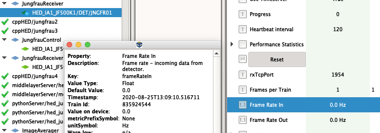
will thus be represented in a measurement HED_IA1_JF500K1/DET/JNGFR01 under the field frameRateIn-FLOAT in InfluxDB and thus Grafana:

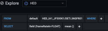
Since device name uniqueness is guaranteed for each Karabo topic, and measurement name uniqueness must be assured in InfluxDB, each Karabo topic stores its logging data in a dedicated Influx database named after the topic. In the example above this is HED.

Data Type Support

All Slow Control Karabo data types are supported by the InfluxDB loggers.

However, Karabo has a few datatypes which are not represented well by InfluxDB native types, or have limitations in being displayed in Grafana. The below list indicates current support and limitations:

Floating Point:the float and double data types are handled by the native floating point type of InfluxDB and will display as expected in Grafana. Integer:types are represented by the native integer type of InfluxDB. The will display as expected in Grafana. There is a minor exception in that Influx does not support uint64`(`unsigned long long) data types. We thus cast this type to the supported int64 type. This will lead extremely large numbers, which use the 63rd bit, being displayed negative in Grafana. This problem is foreseen to occur very rarely, if at all. Boolean:types are converted to 0 (false) and 1 (true) and display as such in Grafana Strings:are stored as strings and display as such in Grafana. Note that for strings the aggregate function set is greatly reduced in InfluxDB, e.g. you cannot aggregate strings to a mean or max value. However, counting the occurance of (distinct) strings is possible. Strings best display in the table display widged of Grafana. Vectors:are serialized into a base64-encoded string form. Their content is thus opaque to InfluxDB and Grafana. However, counting the number of distinct occurances can be useful in some scenarios, such as for the bunch pattern table.

Creating Panels and Visualizations

Creating a panel and the available visualizations are well described in the Grafana Documentation: https://grafana.com/docs/grafana/latest/panels/add-a-panel/, and https://grafana.com/docs/grafana/latest/panels/visualizations/. Make sure to check the menu on the left of these pages for chapters with detailed information.

Examples

Quick Inspection of a Vacuum Incident

On the morning of February 4th 2020 the SPB_EHC_VAC/VALVE/VALVE_ROUGH_1 which is part of the AGIPD vacuum system was found in an UNKNOWN state. To investigate we want to plot related pressure values from the archive.

Since initially we want to check what data might be useful we choose not to create a panel or even dashboard right away. Rather, we use the Explore feature of Grafana, which allows for ad-hoc investigations.

We thus click on the “Compass” icon in the menu, which opens an ad-hoc panel.

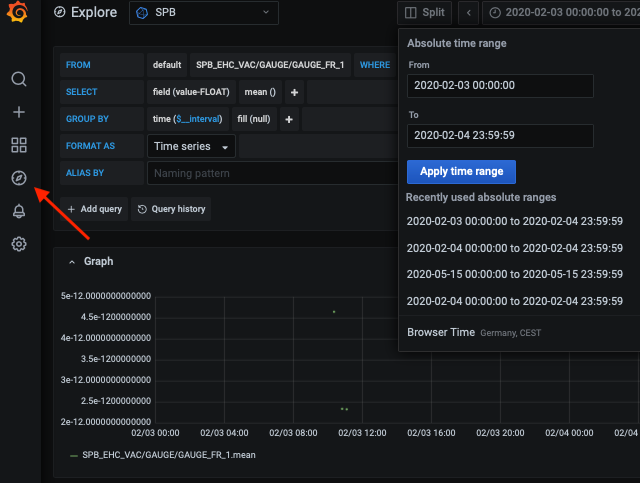
We choose SPB as data source as this corresponds to our Karabo topic. Since we are interested in the EHC component we look for a gauge there and select it as measurement. The pressure itself will be in the value-FLOAT field. Finally we adjust the time range to the period of interested, as should in the screenshot.

We now see the development of the pressure of SPB_EHC_VAC/GAUGE/GAUGE_FR_1. If we are interested in the other gauges tracking pressures in the EHC component, we could add more queries using the Add Query button. However, **using a Regular Expression* we can avoid this repetitive work.

Measurements can be given as regular expressions, so instead of SPB_EHC_VAC/GAUGE/GAUGE_FR_1 we can write /SPB_EHC_VAC/GAUGE/GAUGE.*/ which will plot the value-FLOAT field from all devices which start with SPB_EHC_VAC/GAUGE/GAUGE. Note how in InfluxDB a regular expression is enclosed in /. Also not that we need to escape the slashes in the device name, i.e. use /. Our plot will now look like

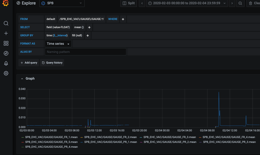
We now see that there were spikes in pressure and also that for a longer period in the night the vacuum system was in a state where no logging information was recieved. This might have to do with the observed UNNOWN state.

Hence, to recover when the detector powered down, we need additional information. We decided to check the logs of the power supplies which should trip in case of a vacuum incident.

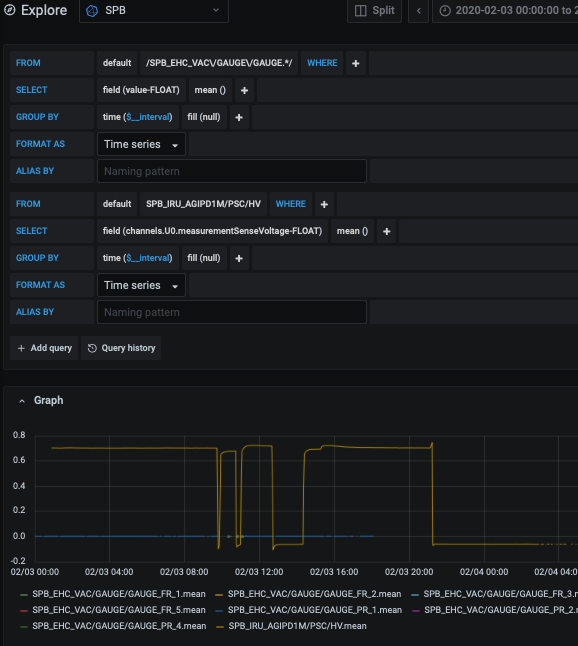
To do so we click Add Query and add the MPOD device controlling the high voltage of AGIPD: SPB_IRU_AGIPD1M/PSC/HV. The interesting values are the sense voltages, so we select this as field from channel 0: channels.U0.measurementSenseVoltage-FLOAT. This already shows us some correlation between the pressure behaviour and the voltage. Especially, we can see that the detector tripped or was powered down around 21.00 on Feb. 3rd.

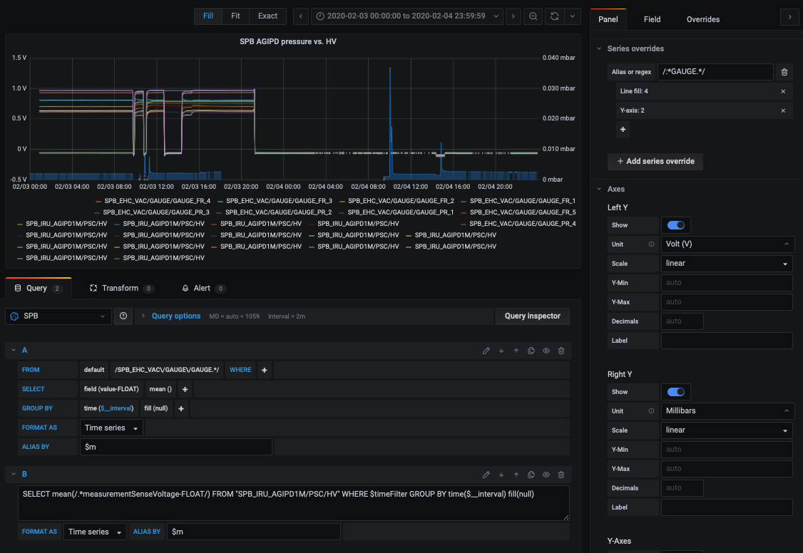
To verify we decide to plot voltage trends for all HV channels. Again, we could add more queries manually, but decide to use a regular expression instead. For this we switch into textual query mode by clicking on the pen icon. This allows us to edit the query we’ve previously defined through the grafical editor:

SELECT mean(/.*measurementSenseVoltage-FLOAT/) FROM "SPB_IRU_AGIPD1M/PSC/HV" WHERE $timeFilter GROUP BY time($__interval) fill(null)

Here the important part is the regex in the mean`function, which follows the same pattern as we used for the pressure value. The regex is enclosed in `/, and via .* we allow any field to be evaluated which ends with measurementSenseVoltage-FLOAT.

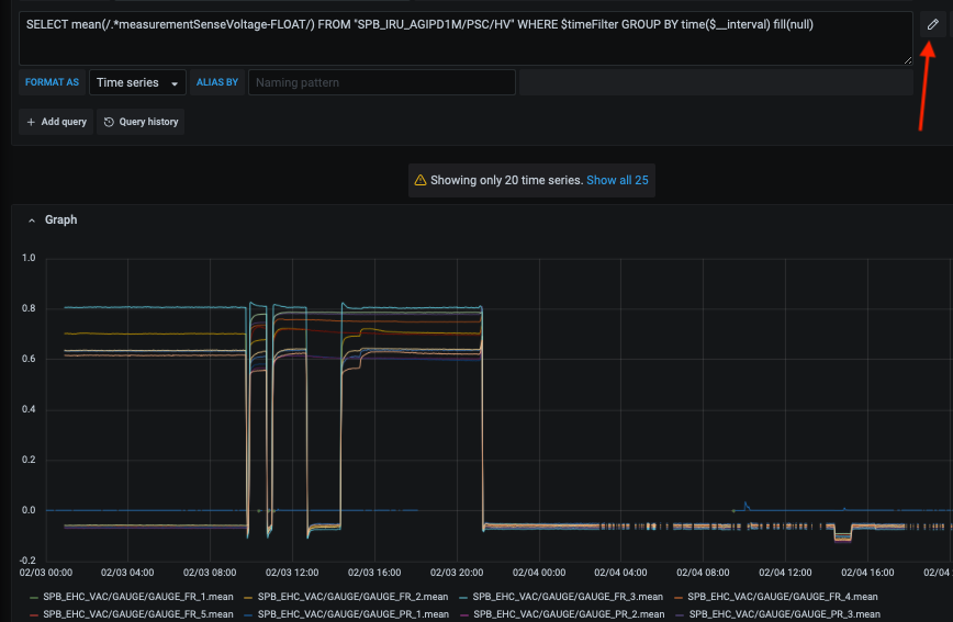
We can now see that all channels exhibited similar behaviour at the same time. However, we also observe that the value ranges of pressure and voltage are too different to display well on a single y-axis. Rather, two axes would be beneficial. We cannot do this in the Explore view, but since we consider the panel useful for future events we decide to create a proper dashboard with panel.

Using Two Y-axes

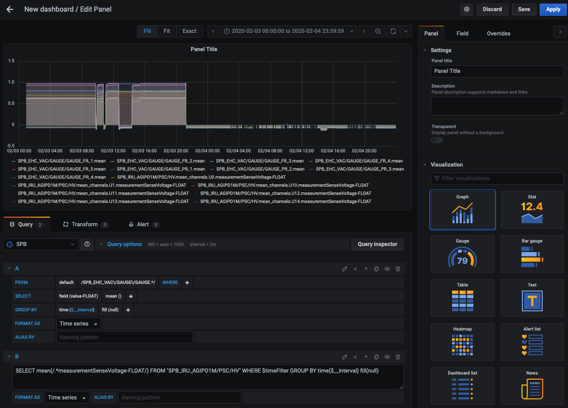
In this example we convert the preliminary investigation of the previous example, Quick Inspection of a Vacuum Incident, into a panel on a dashboard and adjust it to have two y-axes. This will allow us to display in the same plot values with divergent y-values.

We start by creating a new dashboard in the Detector folder. We then add a New Panel on the following screen, and enter the two queries from the previous example. Setting the time period to Feb 4th again, we should get something like the following:

Our primary goal is to add a second y-axis to have a better display of pressure and voltages in the same plot. For this we scroll down the right Panel to Series overrides (https://grafana.com/docs/grafana/latest/panels/visualizations/graph-panel/#series-overrides). Here we can assign a separate y-axis to our pressure data. For this we identfiy the data which is to have its axis overwritten via a regular expression. We know the pressure device/measurement names will contain GAUGE, while the voltage measurements will not. Hence, /:*GAUGE.*/ is a suitable expression. We can then click on the + icon to add an override for the y-axis:

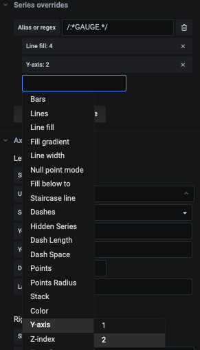
To further improve display, we make a few more changes: we set the line fill in the main options to 0 but override it for pressure with 4. Additionally, we add units to the Axes: Energy->Volt(V) for Left Y and Pressure -> Millibars for Right Y. Finally, we add $m to the ALIAS BY field of our queries. This will shorten the legend entries to the measurment name only (https://grafana.com/docs/grafana/latest/features/datasources/influxdb/#alias-patterns).

Our plot should now look similar to the following:

We could now parameterise the panel via Dashboard variable to e.g. make it useful for the MID AGIPD as well. See :ref:`db_variables`_ for an example on this.

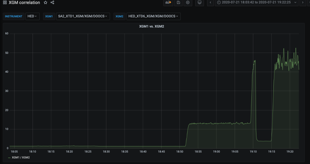
Correlate two XGMS

In this example we correlate the intensities recorded by two XGMs in the same SASE. The data shown here is from an EPIX irradiation beamtime in August 2020. For this it was of interest how the SA1_XTD1_XGM and the HED_XTD6_XGM correlate in the photon energy they register per train. The panel we will be discussing in the following is available in General->XGM correlation and parameterised for all instruments (not all have two XGMs though). It looks like this for the time period we will evaluate in the example:

Let’s recreate it step by step. We start by adding the relevant queries (see examples above). Note that in the screenshot these are parameterised bia an $INSTRUMENT variable referring to the database, and regexes on $XGM1`and `$XGM2 variables referring to the measurements of the to-be-correlated XGMs.

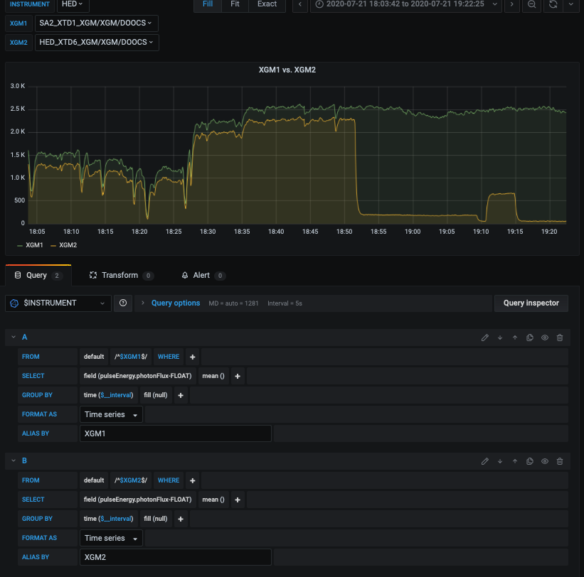
The regex is necessary as the $XGM1/2 variable is defined as a query variable which shows all measurements matching an expression /.*DOOCS.*XGM/.

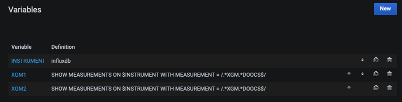
This would also match the _events and _schema internal measurements, which we reject by defining that there cannot be any characters before or after the variable’s content: /^$XGM1$/, where ^ is the start of the field entry and $ its end.

Note that currently we simply have two series in our plot. However, we would like to have their correlation, i.e. in terms of XGM1’s recorded energy with respect to XGM2’s. We can do this using Grafana`s Transform feature:

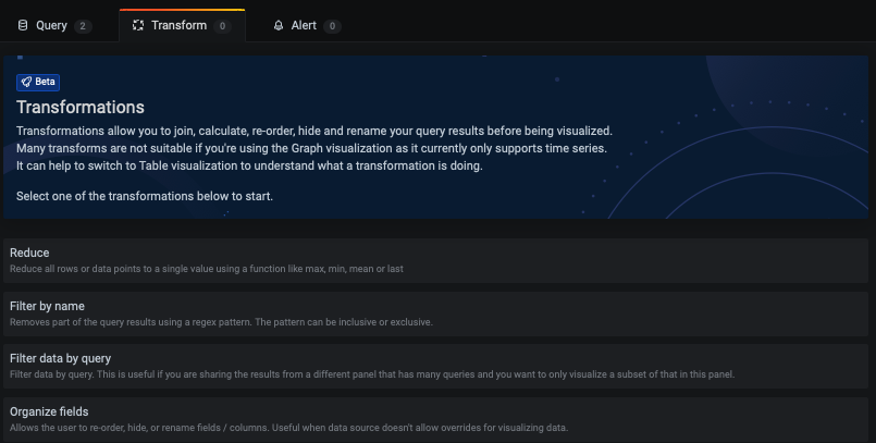
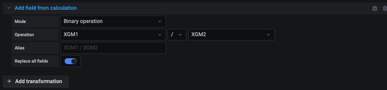
There are many different transforms to select from, which are documented here: https://grafana.com/docs/grafana/latest/panels/transformations/. Interesting for us is Add field from calculation which is described as use the row values to calculate a new field. We thus select this and the select Binary operation as Mode. We can now enter the operation as XGM1 / XGM2. Importantly, we select Replace all fields to hide the original data series and display only the calculated value:

Displaying String Fields - Karabo Device States

For string fields many of the aggregate functions are not defined. Consider e.g. what the mean value of a string should be. However, there are a few useful visualizations Grafana can provide for string fields, and here most importantly Karabo device states.

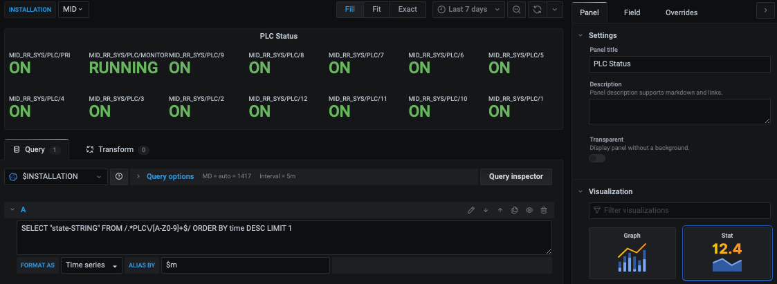
Displaying the current State of a device can be done via a query which orders by time and only retrieves the latest result, e.g.

SELECT "state-STRING" FROM /.*PLC\/[A-Z0-9]+$/ ORDER BY time DESC LIMIT 1

will retrieve the current state of all PLCs in a database/Karabo topic. A good visualization option for this is the Stat graph:

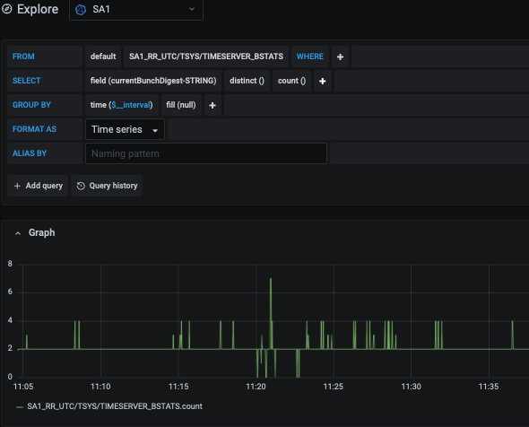
To evaluate the number of state updates a device has in a given time period, i.e. to check if a digital output is “flickering”, we can evaluate the number (count) of discrete values. This is also useful to check how often a bunch pattern changes, where each pattern is stored in a string-encoded hash: