7. pnCCD Data Acquisition
7.1. Run Control
The SQS DAQ Karabo subproject is called SQS_DAQ_RUN_MGMT, which is found under the AMAIN main project. Click on the little triangle beside the SQS_DAQ_RUN_MGMT subproject to expand it. Open the SQS_RUN_CONTROL_GLOBAL_STATE scene (Fig. 7.1).
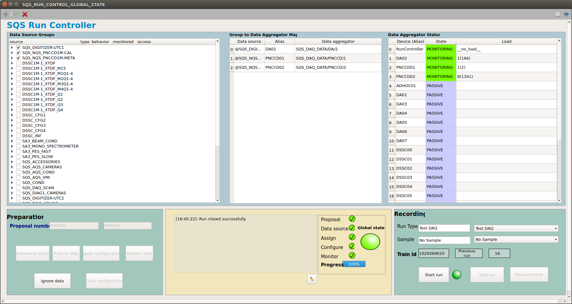
Fig. 7.1 The SQS_RUN_CONTROL_GLOBAL_STATE scene with which one can set up the run control. Here, only the data sources related to the pnCCD devices are selected.
To set up the DAQ in order to take a data run with pnCCD:
Make sure that detector is in acquiring mode. If so, the
ADC 1andADC 2states are both inAcquiringmode on thepnCCD_Mainscene (see Fig. 6.2).If a run is not currently in progress, click on the
Ignore databutton (see Fig. 7.1). This step is only necessary if you want to change the proposal number and/or the data sources. With this step, the DAQ will go into theIgnorestate.From the
Data Source Groupsfield (see Fig. 7.1), select, by clicking on the little square on their left hand side, the pnCCD data aggregators, which are:SQS_NQS_PNCCD1M-CALSQS_NQS_PNCCD1M-METASQS_DIGITIZER-UTC1: This is required only if you need to use Karabo bridge.- The three abovementioned data sources are sufficient for pnCCD. If the experiment requires some other data sources from SQS devices other than pnCCD, make sure their corresponding data sources are also selected. The SQS beamline scientists should be able to assist you in identifying these latter data sources if you are unsure which ones to select.
Click on the green check mark (Apply All Changes) on the top left corner of the
SQS_RUN_CONTROL_GLOBAL_STATEscene to apply the changes. At this point, theData sourceboolean state indicator (resembels a small LED on the bottom middle of Fig. 7.1) should be green.Write the desired proposal number in the corresponding field in the
SQS_RUN_CONTROL_GLOBAL_STATEscene (see Fig. 7.1) and hitEnter(keyboard return). Click onRetrieve Proposalbutton. TheProposalboolean state indicator (resembels a small LED on the bottom middle of Fig. 7.1) should now also be green.Click on the
Push to DAQbutton on theSQS_RUN_CONTROL_GLOBAL_STATEscene. Wait a few seconds. TheAssignboolean state indicator should now be green.Click on
Apply configurationbutton and wait until the status message bar (on the middle bottom of Fig. 7.1) confirms that the application was successful. TheConfigureboolean state indicator should now be green.Click on
Monitor databutton on theSQS_RUN_CONTROL_GLOBAL_STATEscene and ensure theMonitorboolean state indicator also turns green.At this point, the
Progressbar should be green and should show 100 percent. if everything has worked like it should, the big boolean state LED indicator calledGloabal Stateshould be green.If you want to take a dark run, choose “Dark Run for Gain xxx” (specify which gain setting it is for) as the
Run Typeand choose “No Sample” for theSamplefield (see Fig. 7.1). If these are not available, please ask an SQS beamline scientist to make them using the Meta Data Catalog so that the dark runs can be labeled correctly. Everytime you make a change, click on the keyboard return key to ensure that your change is saved in Karabo. If the run is not a dark one, choose appropriate names forRun TypeandSamplefields.Follow the instructions given in
DarkRunsto start a dark run.After enough data are saved (for example, 500 trains are enough for a dark run), click on
Stop runbutton (see Fig. 7.1) to stop the run.
7.2. Offline Data
Following the instructions given in the previous section, raw data are saved on disk.
7.2.1. Accessing the Raw Data
To access the raw data, follow these steps:
Make sure you have permission to access the proposal under study. If not, ask the SQS beamline scientists to add your username to the desired proposal if possible.
Connect to the Maxwell cluster (you may need to first connect to
bastion.desy.de):ssh -XY username@max-exfl
Go to the directory where the current raw data are being stored:
cd /gpfs/exfel/exp/SQS/201921/p002430/raw/r0010Here, the syntax is as follows:
SQSis the instrument.201921is the cycle number.p002430is the proposal number.r0010means the desired run number is 10.
If the DAQ is setup correctly and the connection between the DAQ device and the data aggregators is established correctly, for run number
XXX, there should be a few files in ther0XXXdirectory. Depending on the selected data sources, these files are of three types:- Files like
RAW-R0XXX-DA##-S000##.h5 - Files like
RAW-R0XXX-PNCCD01-S000##.h5 - Files like
RAW-R0XXX-PNCCD02-S000##.h5
- Files like
where DA## or PNCCD## refers to the data aggregators, and S000## refers to the file sequence. Roughly, every 500 trains consists of one sequence. Therefore, if the duration of the run corresponds to 1500 trains, you will end up with 3 raw data files per each selected data aggregator. Note that there will be one image frame saved per train. Also, the slow data are saved in the PNCCD02 data files, while the fast data are saved in the PNCCD01 data files. The slow data refer to the pnCCD gain, bias voltages (HV values for top and bottom pnCCD modules) and the sensors’ temperatures. The fast data are the pnCCD image arrays.
Note
- Only those files whose names contain
PNCCD01orPNCCD02will have the data collected by the pnCCD detector because only these files are generated by the correct pnCCD data aggregators.
To open a raw data file, which contains the pnCCD fast data, on Maxwell cluster, do the following:
1
2
module load xray
hdfview3 RAW-R0XXX-PNCCD01-S000##.h5
Go to
Openmenu (looks like an open book with a red arrow pointing downwards) and click on the menu button found on the top looking like a box with a black square and a ring inside. Browse togpfsfolder and then browse to your desired raw data file.A window opens, which should have the complete path of your desired raw data file in
Recent Filesbox. Browse to the following path to have access to the raw image data:/INSTRUMENT/SQS_NQS_PNCCD1MP/CAL/PNCCD_FMT-0:output/data/image/
To ensure data is being properly written on the disk, make sure that the
imageis non empty and non zero. To do this, one has to display the data and ensure the size of the data array is \(x \times 1024 \times 1024\), where \(x\) is the number of frames and \(0 < x \leq 500\). To display the raw data:- Double click on the
imageto open the raw data image as an array in a spreadsheet. - To visualize the data as 2D images (see Fig. 7.2 and Fig. 7.3), right click on the
imagein the above mentioned path and click onOpen As. A window pops up. SelectImageas display type. Select the desired color scale from theSelect palettedrop-down menu. If desired, choose a valid range by setting the desired minimum and maximum ADU values. SetHeightas dimension 1 (1024 pixels) andWidthas dimension 2 (1024 pixels).Depthwould be dimension 0 which is the number of available frames. Click onResetto set theDepth-Endto the maximum available number of frames. Now, you can also change the frame to be displayed (default is frame 0). Finally, pressOKto display the image. Once the image is shown, one can choose to display various frames by using the forward and backward arrows.
- Double click on the
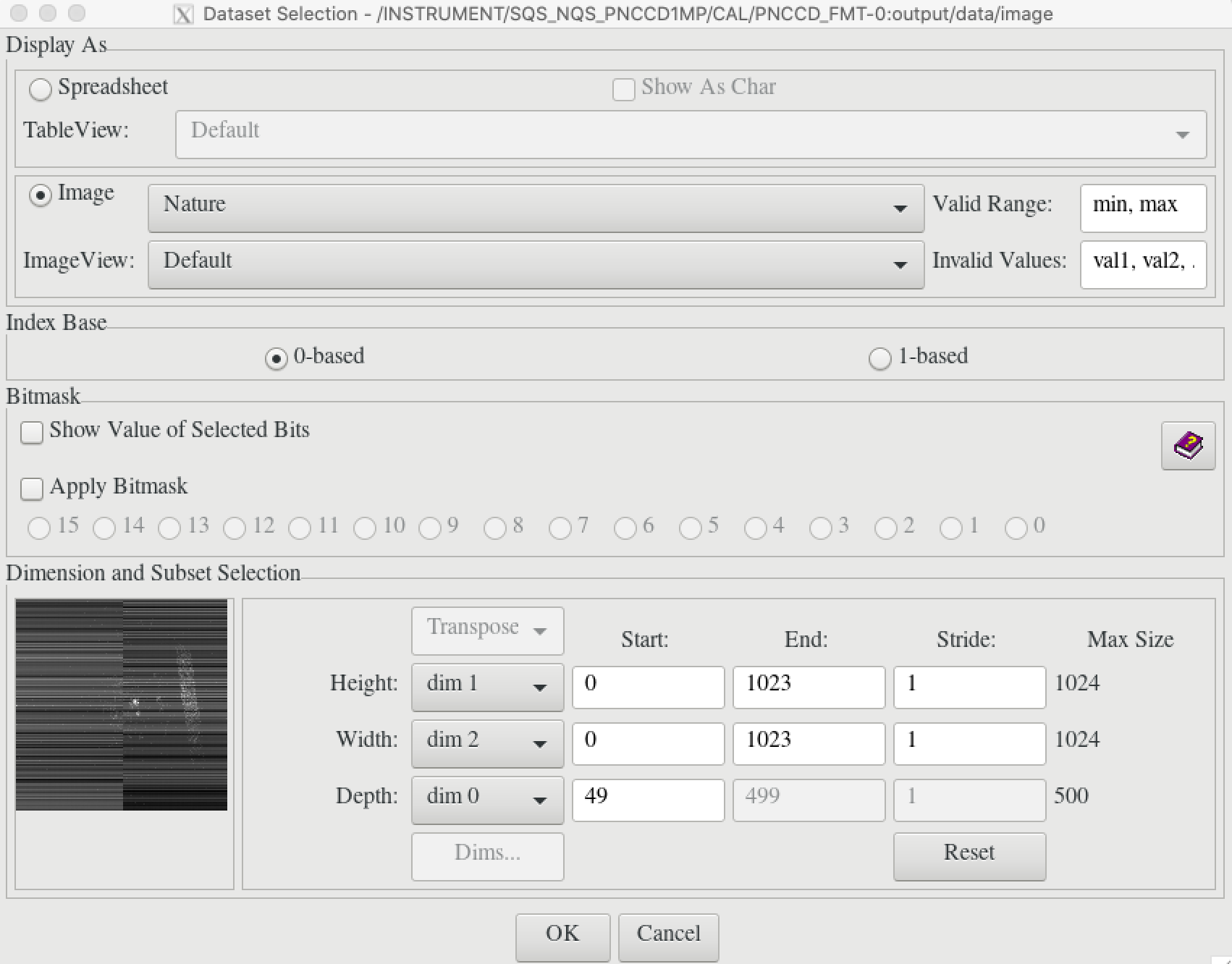
Fig. 7.2 Setting up hdfview3 to display the raw image data.
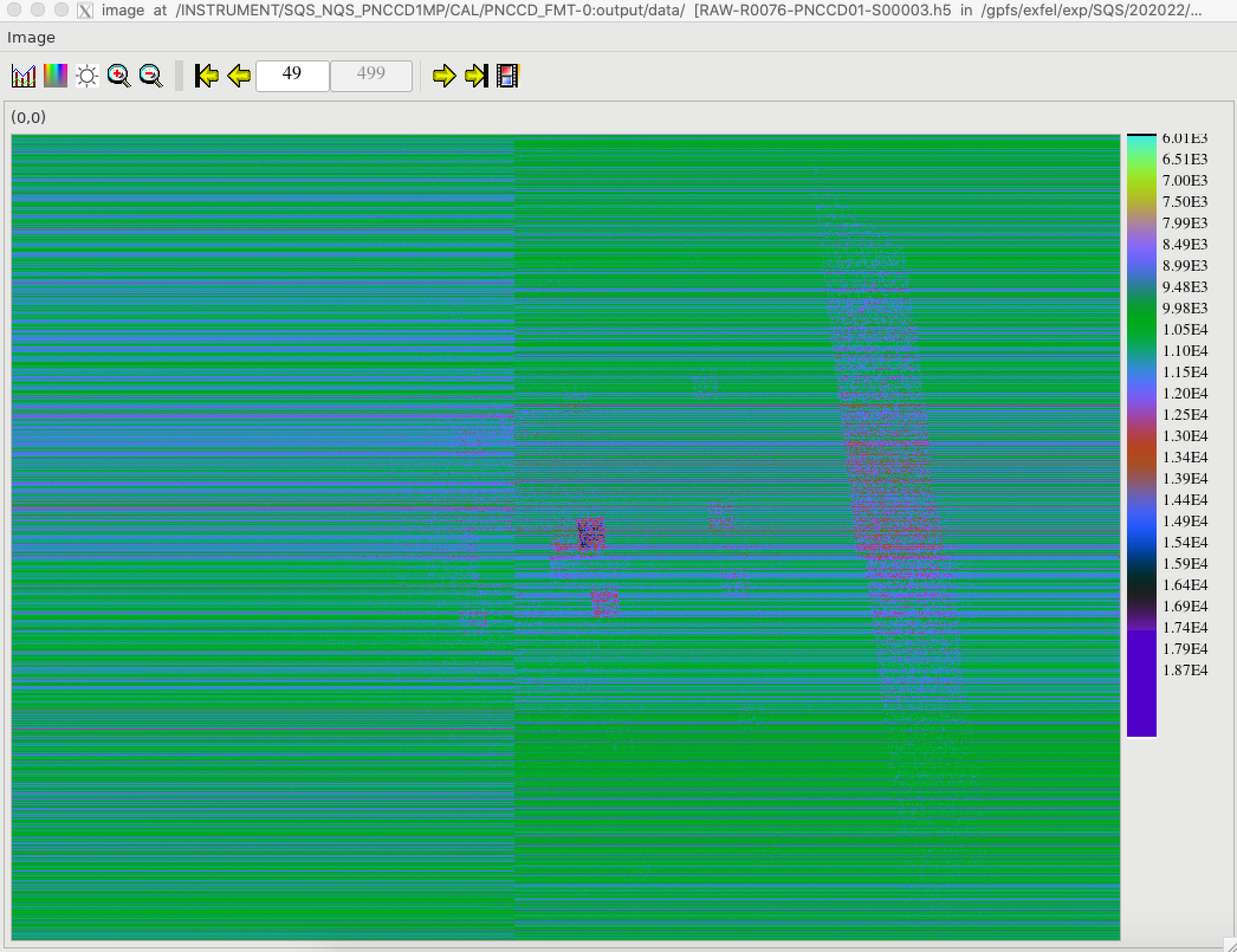
Fig. 7.3 The raw image data using the hdfview3 tool. The image that is shown here is only part of the actual image due to the limitation of the size of my remote desktop display. What is plotted is sequence 3 of run 76 from proposal p002720 from cycle 202022. The displayed image is frame 49 out of 500 available images and shows the scattered X-rays from a membrane with a lot of small holes.