Analysis of Viking spectrometer data
The Viking spectrometer is typically used with an Andor Newton CCD to record the transmitted FEL spectrum. The Viking class of the SCS ToolBox contains all the details about the experiment, but no data. It allows the calculation of an absorption spectrum based on averaged spectra with and without sample (reference).
All the parameters need to be carefully calibrated whenever the spectrometer is moved, usually at the beginning of a beamtime.
[1]:
%load_ext autoreload
%autoreload 2
[2]:
import numpy as np
import xarray as xr
import matplotlib.pyplot as plt
plt.rcParams['figure.constrained_layout.use'] = True
#%matplotlib notebook
import toolbox_scs as tb
Setting the stage
[3]:
proposal = 2953
runNB = 321  # run containing the data with sample
refNB = 322  # run containing the data without sample
darkNB = 375  # dark run
[4]:
v = tb.Viking(proposal)
v.FIELDS += ['XTD10_SA3']  # add the pulse energy measured by XGM in the XTD10 tunnel
v.X_RANGE = slice(0, 1500) # define the dispersive axis range of interest (in pixels)
v.Y_RANGE = slice(29, 82) # define the non-dispersive axis range of interest (in pixels)
v.ENERGY_CALIB = [1.47802667e-06, 2.30600328e-02, 5.15884589e+02] # energy calibration, see further below
v.BL_POLY_DEG = 1 # define the polynomial degree for baseline subtraction
v.BL_SIGNAL_RANGE = [500, 545] # define the range containing the signal, to be excluded for baseline subtraction

v.load_dark(darkNB)  # load a dark image (averaged over the dark run number)
Loading data
[5]:
ds_ref = v.from_run(refNB)  # load refNB. The `newton` variable contains the CCD images.
v.integrate(ds_ref)  # integrate over the non-dispersive dimension
v.removePolyBaseline(ds_ref)  # remove baseline
ds_ref
[5]:
<xarray.Dataset>
Dimensions:            (newt_x: 1500, newt_y: 53, pulse_slot: 2700, sa3_pId: 43, trainId: 661)
Coordinates:
  * trainId            (trainId) uint64 1473952798 1473952800 ... 1473954118
  * sa3_pId            (sa3_pId) int64 1056 1088 1120 1152 ... 2336 2368 2400
  * newt_x             (newt_x) float64 515.9 515.9 515.9 ... 553.7 553.7 553.8
Dimensions without coordinates: newt_y, pulse_slot
Data variables:
    bunchPatternTable  (trainId, pulse_slot) uint32 2146089 2048 ... 16777216
    newton             (trainId, newt_y, newt_x) float64 943.0 800.0 ... 758.0
    XTD10_SA3          (trainId, sa3_pId) float64 1.674e+03 ... 1.465e+03
    spectrum           (trainId, newt_x) float64 941.8 960.7 ... 1.319e+03
    spectrum_nobl      (trainId, newt_x) float64 -25.84 -7.063 ... -41.9 -25.1
Attributes:
    runFolder:                 /gpfs/exfel/exp/SCS/202202/p002953/raw/r0322
    vbin::                     4
    hbin:                      1
    startX:                    1
    endX:                      2048
    startY:                    1
    endY:                      512
    temperature:               -50.04199981689453
    high_capacity:             0
    exposure_s:                0.0004
    gain:                      2
photoelectrons_per_count: 2.05- newt_x: 1500
- newt_y: 53
- pulse_slot: 2700
- sa3_pId: 43
- trainId: 661
- trainId(trainId)uint641473952798 ... 1473954118
array([1473952798, 1473952800, 1473952802, ..., 1473954114, 1473954116, 1473954118], dtype=uint64) - sa3_pId(sa3_pId)int641056 1088 1120 ... 2336 2368 2400
array([1056, 1088, 1120, 1152, 1184, 1216, 1248, 1280, 1312, 1344, 1376, 1408, 1440, 1472, 1504, 1536, 1568, 1600, 1632, 1664, 1696, 1728, 1760, 1792, 1824, 1856, 1888, 1920, 1952, 1984, 2016, 2048, 2080, 2112, 2144, 2176, 2208, 2240, 2272, 2304, 2336, 2368, 2400]) - newt_x(newt_x)float64515.9 515.9 515.9 ... 553.7 553.8
array([515.884589, 515.907651, 515.930715, ..., 553.717729, 553.745216,
       553.772706])
- bunchPatternTable(trainId, pulse_slot)uint322146089 2048 ... 16777216 16777216
array([[ 2146089, 2048, 2099241, ..., 16777216, 16777216, 16777216], [ 2146089, 2048, 2099241, ..., 16777216, 16777216, 16777216], [ 2211625, 2048, 2099241, ..., 16777216, 16777216, 16777216], ..., [ 2146089, 2048, 2099241, ..., 16777216, 16777216, 16777216], [ 2146089, 2048, 2099241, ..., 16777216, 16777216, 16777216], [ 2146089, 2048, 2099241, ..., 16777216, 16777216, 16777216]], dtype=uint32) - newton(trainId, newt_y, newt_x)float64943.0 800.0 697.0 ... 805.0 758.0
array([[[ 943., 800., 697., ..., 985., 1057., 1038.], [ 842., 921., 957., ..., 1037., 1041., 978.], [ 744., 587., 558., ..., 1094., 925., 1030.], ..., [ 600., 688., 836., ..., 970., 1061., 1204.], [ 681., 625., 675., ..., 921., 938., 887.], [ 695., 593., 822., ..., 666., 582., 829.]], [[ 918., 949., 901., ..., 892., 976., 905.], [ 857., 912., 1083., ..., 731., 757., 758.], [ 630., 575., 599., ..., 1058., 967., 914.], ..., [ 741., 776., 874., ..., 784., 961., 1391.], [ 684., 971., 878., ..., 954., 1218., 1041.], [ 831., 647., 744., ..., 643., 690., 733.]], [[ 634., 709., 727., ..., 985., 963., 836.], [ 553., 612., 787., ..., 1169., 788., 903.], [ 668., 618., 621., ..., 785., 863., 835.], ..., ... ..., [ 920., 815., 759., ..., 844., 1050., 839.], [1080., 956., 661., ..., 968., 1001., 915.], [ 811., 918., 652., ..., 873., 823., 1034.]], [[ 733., 606., 582., ..., 880., 1039., 1139.], [ 784., 806., 787., ..., 1075., 1125., 827.], [ 889., 848., 957., ..., 962., 1071., 811.], ..., [ 860., 649., 578., ..., 962., 1151., 985.], [ 845., 663., 688., ..., 836., 978., 1340.], [ 732., 784., 586., ..., 734., 872., 829.]], [[ 697., 934., 742., ..., 873., 753., 931.], [ 694., 730., 774., ..., 802., 1020., 1206.], [ 697., 956., 694., ..., 700., 785., 899.], ..., [ 799., 717., 918., ..., 898., 951., 1050.], [ 870., 949., 918., ..., 911., 1283., 1080.], [ 894., 627., 652., ..., 1032., 805., 758.]]]) - XTD10_SA3(trainId, sa3_pId)float641.674e+03 1.781e+03 ... 1.465e+03
array([[1673.97485352, 1780.60498047, 1452.16772461, ..., 1836.07592773, 1695.68798828, 1458.07446289], [2012.43261719, 1767.71337891, 1716.76318359, ..., 1651.42553711, 1813.9777832 , 1431.35644531], [1630.87841797, 1645.91479492, 1469.28320312, ..., 1508.0567627 , 1385.63110352, 1416.71606445], ..., [1507.31445312, 1752.1652832 , 1686.92077637, ..., 1737.3125 , 1577.06298828, 1616.52392578], [2101.60083008, 1569.24121094, 1855.71728516, ..., 1483.96960449, 1664.98217773, 1348.71264648], [1564.17675781, 1731.5670166 , 1535.64672852, ..., 1721.94335938, 1681.0324707 , 1465.49145508]]) - spectrum(trainId, newt_x)float64941.8 960.7 ... 1.302e+03 1.319e+03
array([[ 941.7582056 , 960.74608693, 985.17661157, ..., 1429.04862315, 1345.94592645, 1329.10501995], [1078.21858296, 1053.6536341 , 1074.17755497, ..., 1328.01843447, 1424.27139815, 1363.56822749], [ 935.14405465, 949.06495485, 981.38604553, ..., 1409.16749108, 1329.46856796, 1194.42388787], ..., [1025.26669616, 1002.32627561, 985.83415874, ..., 1286.786359 , 1334.07139815, 1294.75785014], [1083.24688484, 1097.98004919, 1044.16246063, ..., 1231.70711372, 1391.47139815, 1360.74464259], [1022.09499805, 1066.14703033, 1049.92566818, ..., 1362.59767976, 1302.00630381, 1319.00973693]]) - spectrum_nobl(trainId, newt_x)float64-25.84 -7.063 17.16 ... -41.9 -25.1
array([[ -25.83894992,   -7.0628976 ,   17.15577088, ...,  113.9392577 ,
          30.58408468,   13.49067472],
       [ 132.95041047,  108.12852617,  128.39547866, ...,  -38.76048694,
          57.18623863,   -3.82320306],
       [  -4.23392908,    9.48766827,   41.60943055, ...,  142.82685757,
          62.89038791,  -72.39186427],
       ...,
       [  22.22161966,   -0.8666322 ,  -17.50659932, ...,   41.21934094,
          88.32818182,   48.83841661],
       [  80.40434786,   94.90808737,   40.86104455, ..., -147.51415939,
          11.97667647,  -19.02355706],
       [ -34.85541266,    9.02183124,   -7.3743417 , ...,   18.90138573,
         -41.89831828,  -25.10323562]])
- runFolder :
- /gpfs/exfel/exp/SCS/202202/p002953/raw/r0322
- vbin: :
- 4
- hbin :
- 1
- startX :
- 1
- endX :
- 2048
- startY :
- 1
- endY :
- 512
- temperature :
- -50.04199981689453
- high_capacity :
- 0
- exposure_s :
- 0.0004
- gain :
- 2
- photoelectrons_per_count :
- 2.05
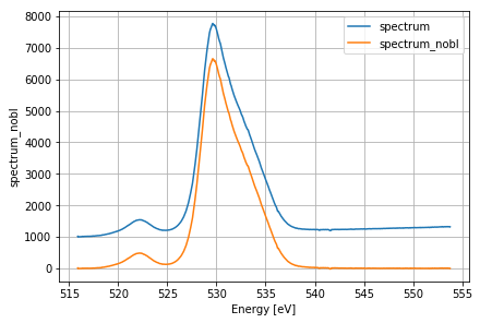
Plotting baseline subtracted spectrum
There is often a broad spectral background added to the SASE spectra that needs to be removed. To do so, a polynomial of degree BL_POLY_DEG is fitted to the baseline. The ranges where the actual SASE signal is present are avoided by setting the BL_SIGNAL_RANGE parameter.
[6]:
plt.figure()
ds_ref['spectrum'].mean(dim='trainId').plot(label='spectrum')
ds_ref['spectrum_nobl'].mean(dim='trainId').plot(label='spectrum_nobl')
plt.legend()
plt.xlabel('Energy [eV]')
plt.grid()
Calculating and plotting XAS spectrum
[7]:
ds = v.from_run(runNB)  # load runNB
v.integrate(ds)  # integrate over the non-dispersive dimension
v.removePolyBaseline(ds)  # remove baseline

xas = v.xas(ds, ds_ref, thickness=1, plot=True, xas_ylim=(-1, 3))
xas
[7]:
<xarray.Dataset>
Dimensions:                (newt_x: 1500)
Coordinates:
  * newt_x                 (newt_x) float64 515.9 515.9 515.9 ... 553.7 553.8
Data variables:
    It                     (newt_x) float64 3.919 -2.476 ... 0.01703 -2.786
    It_std                 (newt_x) float64 46.04 43.49 44.08 ... 33.76 35.61
    It_stderr              (newt_x) float64 1.852 1.75 1.773 ... 1.358 1.433
    I0                     (newt_x) float64 8.241 -13.35 -7.251 ... 1.327 -4.828
    I0_std                 (newt_x) float64 46.04 43.49 44.08 ... 33.76 35.61
    I0_stderr              (newt_x) float64 1.852 1.75 1.773 ... 1.358 1.433
    absorptionCoef         (newt_x) float64 0.7433 1.685 nan ... 4.356 0.5499
    absorptionCoef_std     (newt_x) float64 14.46 18.34 51.7 ... 1.982e+03 16.35
    absorptionCoef_stderr  (newt_x) float64 0.5753 0.7357 2.077 ... 79.73 0.6494
Attributes:
    n_It:     618
n_I0: 661- newt_x: 1500
- newt_x(newt_x)float64515.9 515.9 515.9 ... 553.7 553.8
array([515.884589, 515.907651, 515.930715, ..., 553.717729, 553.745216,
       553.772706])
- It(newt_x)float643.919 -2.476 ... 0.01703 -2.786
array([ 3.91925258, -2.47627339, 0.86810958, ..., 2.20337353, 0.01703439, -2.78575572]) - It_std(newt_x)float6446.04 43.49 44.08 ... 33.76 35.61
array([46.04029465, 43.49329739, 44.08335856, ..., 34.90163389, 33.7584539 , 35.61211943]) - It_stderr(newt_x)float641.852 1.75 1.773 ... 1.358 1.433
array([1.85201226, 1.749557 , 1.77329274, ..., 1.40394961, 1.35796417, 1.43252953]) - I0(newt_x)float648.241 -13.35 ... 1.327 -4.828
array([ 8.24135673, -13.35154356, -7.25066757, ..., 2.16029973, 1.32716927, -4.8278338 ]) - I0_std(newt_x)float6446.04 43.49 44.08 ... 33.76 35.61
array([46.04029465, 43.49329739, 44.08335856, ..., 34.90163389, 33.7584539 , 35.61211943]) - I0_stderr(newt_x)float641.852 1.75 1.773 ... 1.358 1.433
array([1.85201226, 1.749557 , 1.77329274, ..., 1.40394961, 1.35796417, 1.43252953]) - absorptionCoef(newt_x)float640.7433 1.685 nan ... 4.356 0.5499
array([ 0.74326401, 1.68487723, nan, ..., -0.01974263, 4.35556914, 0.54987869]) - absorptionCoef_std(newt_x)float6414.46 18.34 ... 1.982e+03 16.35
array([ 14.46147913, 18.33875578, 51.70064703, ..., 28.2276812 , 1982.11422807, 16.35167582]) - absorptionCoef_stderr(newt_x)float640.5753 0.7357 ... 79.73 0.6494
array([ 0.57525382,  0.73570573,  2.07731818, ...,  1.10989227,
       79.73145801,  0.64938941])
- n_It :
- 618
- n_I0 :
- 661
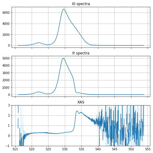
The xas dataset created contains the averaged spectra of the reference I0, of the transmitted signal It, and the absorption coefficient -log(It / I0) / thickness. For each quantity, the standard deviation and standard error are calculated. The number of spectra used in the calculation are added as attributes.
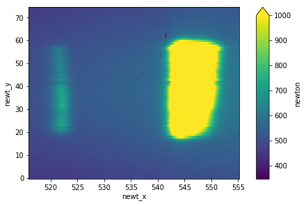
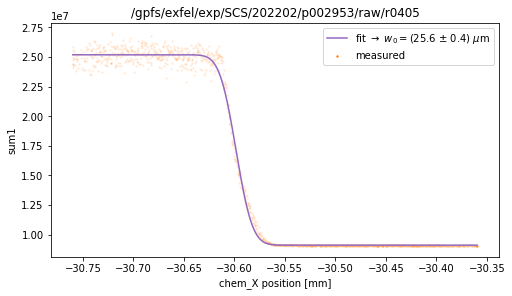
Beam size measurement with knife-edge
[8]:
proposal = 2953
fields = ['newton', 'chem_X']  # chem_X is the manipulator used to move a blade through the beam.

runNB = 405

v.set_params(fields=fields)
v.X_RANGE = slice(0, 1550)
v.Y_RANGE = slice(15, 90)
ds = v.from_run(runNB)
[9]:
plt.figure()
ds['newton'].mean(dim='trainId').plot(vmax=1000)
[9]:
<matplotlib.collections.QuadMesh at 0x2aeb0cbfb828>
[10]:
roi1 = [30, 430]
roi2 = [960, 1540]
ds['sum1'] = ds['newton'].isel(newt_x=slice(*roi1)).sum(dim=['newt_x', 'newt_y'])
ds['sum2'] = ds['newton'].isel(newt_x=slice(*roi2)).sum(dim=['newt_x', 'newt_y'])
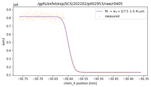
tb.knife_edge(ds, axisKey='chem_X', signalKey='sum1', plot=True) # color 1
tb.knife_edge(ds, axisKey='chem_X', signalKey='sum2', plot=True) # color 2
fitting function: a*erfc(np.sqrt(2)*(x-x0)/w0) + b
w0 = (25.6 +/- 0.4) um
x0 = (-30.598 +/- 0.000) mm
a = 8.038647e+06 +/- 1.638269e+04
b = 9.109166e+06 +/- 2.041594e+04
fitting function: a*erfc(np.sqrt(2)*(x-x0)/w0) + b
w0 = (27.5 +/- 0.4) um
x0 = (-30.598 +/- 0.000) mm
a = 3.405624e+07 +/- 8.242170e+04
b = 1.331917e+07 +/- 1.025471e+05
[10]:
(0.02746726107164219, 0.0004455003530353428)
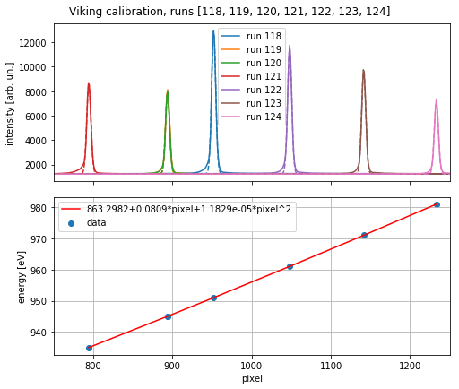
Energy calibration
The calibrate method determines the calibration coefficients to translate the camera pixels into energy in eV. The Viking spectrometer is calibrated using the beamline monochromator: runs with various monochromatized photon energy are recorded and their peak position on the detector are determined by Gaussian fitting. The energy vs. position data is then fitted to a second degree polynomial.
[11]:
proposal = 2593
v = tb.Viking(proposal)
v.X_RANGE = slice(0, 1900)
v.Y_RANGE = slice(30, 75)

print('energy calibration before:', v.ENERGY_CALIB)
runs = list(range(118,125))

v.calibrate(runs, plot=True)
plt.xlim(750, 1250)

print('energy calibration after:', v.ENERGY_CALIB)
energy calibration before: [0, 1, 0]
118
119
120
121
122
123
124
energy calibration after: [1.18294370e-05 8.08628533e-02 8.63298212e+02]