Basic analysis of PES spectra
[1]:
import matplotlib.pyplot as plt
import matplotlib.cm as cm
import numpy as np
import toolbox_scs as tb

proposal = 900447
runNB = 11
Cupy is not installed in this environment, no access to the GPU
Inspect average traces
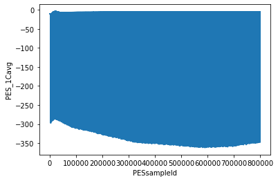
We first load the computed PES average traces that are stored in the proposal folder, under usr/processed_runs. If they do not exist, they can be computed via tb.save_pes_avg_traces(proposal, runNB).
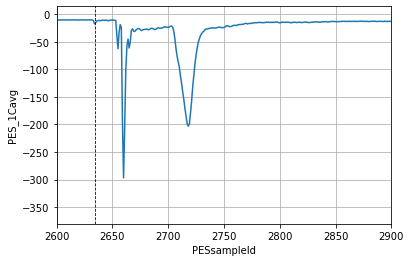
We identify the starting sample of the first spectrum in the raw trace and the location of the prompt which corresponds to the time origin. We get start = 2600 and origin = 2634
[2]:
avg_traces = tb.load_pes_avg_traces(proposal, runNB)
plt.figure()
avg_traces['PES_1Cavg'].plot()

start = 2600
origin = 2634
plt.figure()
avg_traces['PES_1Cavg'].plot()
plt.xlim(start, start + 300)
plt.grid()
plt.axvline(origin, ls='--', color='k', lw=0.8)
[2]:
<matplotlib.lines.Line2D at 0x14da13031c60>
Load PES spectra and other variables
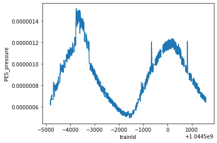
We load the PES pressure and the XTD10 XGM pulse energy, as well as the PES spectra for channel 1C. The function tb.get_pes_tof() extracts each spectrum and aligns the pulse Ids. It also allows merging the resulting PES spectra into the existing dataset (merge_with=ds).
In this case, the raw trace was too short to record all pulses, so the final dataset is truncated to the actual number of pulses recorded.
The dataset contains the time_ns coordinate, calculated using the origin parameter and the digitizer sample rate. The data can be plotted as a function of this coordinate using x='time_ns' argument in the xarray plotting functions.
[3]:
fields = ['PES_pressure', 'XTD10_SA3']
run, ds = tb.load(proposal, runNB, fields)

ds = tb.get_pes_tof(proposal, runNB, 'PES_1Craw',
                    start=start, origin=origin, merge_with=ds)
ds
The digitizer only recorded 453 pulses out of the 579 pulses in the train.
[3]:
<xarray.Dataset> Size: 2GB
Dimensions:            (trainId: 4506, sa3_pId: 453, pulse_slot: 3611,
                        sampleId: 440)
Coordinates:
  * trainId            (trainId) uint64 36kB 2131115942 ... 2131120453
  * sa3_pId            (sa3_pId) int64 4kB 392 396 400 404 ... 2192 2196 2200
  * sampleId           (sampleId) int64 4kB 0 1 2 3 4 5 ... 435 436 437 438 439
    time_ns            (sampleId) float64 4kB -17.12 -16.62 ... 203.4 203.9
Dimensions without coordinates: pulse_slot
Data variables:
    PES_pressure       (trainId) float32 18kB 5.795e-07 5.795e-07 ... 5.704e-07
    bunchPatternTable  (trainId, pulse_slot) uint32 65MB 2113385 0 ... 16777216
    XTD10_SA3          (trainId, sa3_pId) float32 8MB 2.303e+03 ... 2.403e+03
    PES_1Cspectrum     (trainId, sa3_pId, sampleId) int16 2GB -8 -11 ... -10 -7
Attributes:
    runNB:     11
    proposal:  /gpfs/exfel/exp/SA3/202431/p900447
data: allPlot pulse-resolved average over the trains
[4]:
stride = 25
colors = cm.plasma(np.linspace(0, 0.9, int(ds.sizes['sa3_pId']/stride)+1))
s_mean = ds['PES_1Cspectrum'].mean('trainId')

plt.figure(figsize=(12,6))
for i, pid in enumerate(ds.sa3_pId[::stride]):
    s_mean.sel(sa3_pId=pid).plot(x='time_ns',label=i*stride, color=colors[i])
plt.legend(ncol=3, fontsize=12)
plt.xlim(-10, 80)
[4]:
(-10.0, 80.0)
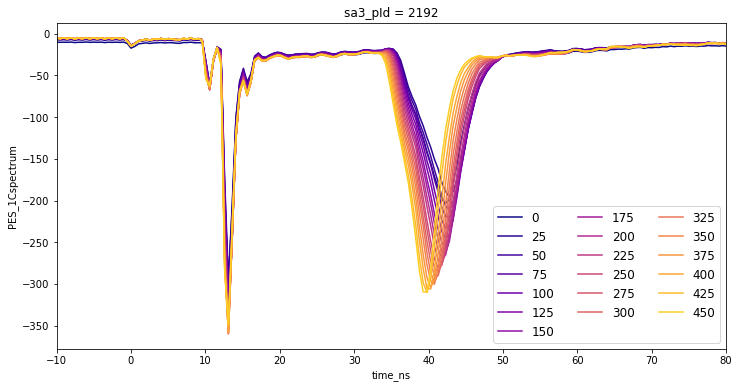
We see that the spectrum shifts and its intensity grows with the number of pulses.
PES calibration
The calibration of the PES involves the gas binding energy, the retardation voltage and other parameters. The first two can be accessed via the tb.get_pes_params() function.
[5]:
def calib(tof, rv):
    return be - rv + PR +(PL/(tof-PT))**2
[6]:
params = tb.get_pes_params(run)
params
[6]:
{'gas': 'N2',
 'binding_energy': 409.9,
 '1A_RV': -111.13424,
 '1B_RV': -111.13424,
 '1C_RV': -111.13124,
 '1D_RV': -111.13424,
 '2A_RV': -111.13124,
 '2B_RV': -111.13401,
 '2C_RV': -111.13124,
 '2D_RV': -111.13124,
 '3A_RV': -111.13401,
 '3B_RV': -111.13401,
 '3C_RV': -111.13424,
 '3D_RV': -111.13401,
 '4A_RV': -111.14254,
 '4B_RV': -111.14254,
 '4C_RV': -111.14254,
 '4D_RV': -111.14254}
We calibrate the energy and add it as a coordinate to the dataset. We also select the region where the energy axis is meaningful (where time is positive and energy < 550 eV).
[7]:
PR = -2.886
PL = 137.24
PT = 7.6
rv = params['1C_RV']
be = params['binding_energy']

ds = ds.assign_coords(energy=('sampleId', calib(ds.time_ns.values, rv)))
ds
[7]:
<xarray.Dataset> Size: 2GB
Dimensions:            (trainId: 4506, sa3_pId: 453, pulse_slot: 3611,
                        sampleId: 440)
Coordinates:
  * trainId            (trainId) uint64 36kB 2131115942 ... 2131120453
  * sa3_pId            (sa3_pId) int64 4kB 392 396 400 404 ... 2192 2196 2200
  * sampleId           (sampleId) int64 4kB 0 1 2 3 4 5 ... 435 436 437 438 439
    time_ns            (sampleId) float64 4kB -17.12 -16.62 ... 203.4 203.9
    energy             (sampleId) float64 4kB 549.0 550.3 551.6 ... 518.6 518.6
Dimensions without coordinates: pulse_slot
Data variables:
    PES_pressure       (trainId) float32 18kB 5.795e-07 5.795e-07 ... 5.704e-07
    bunchPatternTable  (trainId, pulse_slot) uint32 65MB 2113385 0 ... 16777216
    XTD10_SA3          (trainId, sa3_pId) float32 8MB 2.303e+03 ... 2.403e+03
    PES_1Cspectrum     (trainId, sa3_pId, sampleId) int16 2GB -8 -11 ... -10 -7
Attributes:
    runNB:     11
    proposal:  /gpfs/exfel/exp/SA3/202431/p900447
data: all[8]:
spectra = ds['PES_1Cspectrum']
spectra = spectra.where(spectra.energy <=550, drop=True)
spectra = spectra.where(spectra.time_ns >= 0, drop=True)
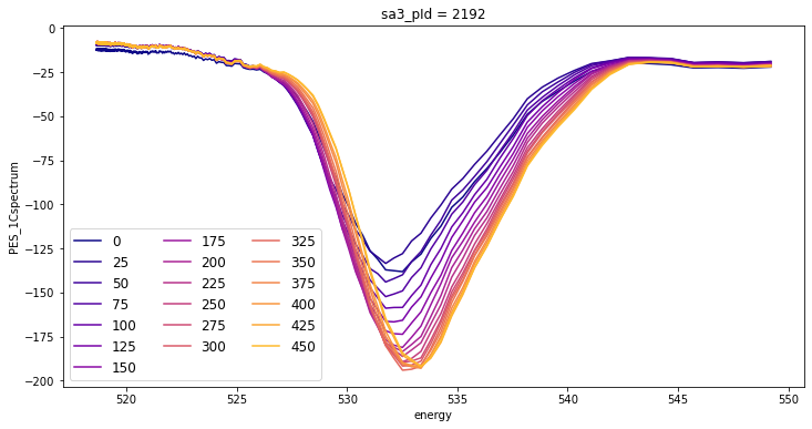
[9]:
stride = 25
colors = cm.plasma(np.linspace(0, 0.85, int(spectra.sizes['sa3_pId']/stride)+1))
s_mean = spectra.mean('trainId')

plt.figure(figsize=(12,6))
for i, pid in enumerate(spectra.sa3_pId[::stride]):
    s_mean.sel(sa3_pId=pid).plot(x='energy',label=i*stride, color=colors[i])
plt.legend(ncol=3, fontsize=12)
[9]:
<matplotlib.legend.Legend at 0x14da0ad3bca0>
The drift in photon energy accross the train is substantial. This was due to a drift in the electron energy on the order of 30 MeV, and was corrected afterwards. This can be seen in the next run:
[10]:
runNB = 12
pes = tb.get_pes_tof(proposal, runNB, 'PES_1Craw',
                     start=start, origin=origin)
pes = pes.assign_coords(energy=('sampleId', calib(pes.time_ns.values, rv)))
pes = pes.where(pes.energy <=550, drop=True).where(pes.time_ns >= 0, drop=True)
pes = pes.sortby('energy')

stride = 25
colors = cm.plasma(np.linspace(0, 0.85, int(pes.sizes['sa3_pId']/stride)+1))
s_mean = pes.mean('trainId')
plt.figure(figsize=(12,6))
for i, pid in enumerate(pes.sa3_pId[::stride]):
    s_mean.sel(sa3_pId=pid).plot(x='energy',label=i*stride, color=colors[i])
plt.legend(ncol=3, fontsize=12)
The digitizer only recorded 453 pulses out of the 577 pulses in the train.
[10]:
<matplotlib.legend.Legend at 0x14da0aee7be0>
[ ]: