Transient optical laser reflectivity measurement: finding FEL and OL time overlap
Transient optical laser reflectivity is a technique to determine the temporal overlap between the FEL and the optical laser (OL). The FEL is pumping a large band gap material (usually a 1 micrometer thick Si\(_3\)N\(_4\) membrane) and the OL, spatially overlaped with the FEL, is reflected off the sample. The incoming (\(I_0\)) and reflected (\(I_r\)) laser beams are monitored by photodiodes. The FEL pump alters the electronic properties of the material, which in turn modifies the reflectivity. By varying the delay between OL and FEL through the scanning of the optical delay line, the transient response of the material is measured and the exact time overlap between the two beams can be extracted.
To increase the signal to noise ratio, pumped and unpumped signals acquired closely in time are compared. The reflectivity is then defined as:
\(\Delta R [\%] = 100\times(\frac{R(pumped)}{R(unpumped)} - 1)\), with \(R = I_r / I_0\)
In the toolbox_scs, there is a convenience function reflectivity that allows the quick calculation of \(\Delta R\). It performs binning along the motor position axis and sorts the data according to the bunch pattern and the sequence of pumped, unpumped.
Below is an example, where \(I_0\) (\(I_r\)) is measured a by photodiode on the Fast ADC channel 5 (channel 3), respectively. The pump FEL is set at half the repetition rate of the OL, to have alternating pumped/unpumped/pumped/unpumped/… pulses within each train.
[1]:
import toolbox_scs as tb
proposal, runNB = 2769, 425
fields = ['FastADC5raw', 'FastADC3raw', 'PP800_DelayLine', 'BAM1932S']
run, ds = tb.load(proposal, runNB, fields)

refl = tb.reflectivity(ds, Iokey='FastADC5peaks', Irkey='FastADC3peaks',
                       delaykey='PP800_DelayLine',
                       binWidth=0.01, plot=True)
refl
[1]:
<xarray.Dataset>
Dimensions:                 (delay: 133)
Coordinates:
  * delay                   (delay) float64 228.2 228.2 228.2 ... 229.5 229.5
Data variables:
    FastADC5peaks           (delay) float64 2.009e+05 1.958e+05 ... 1.937e+05
    FastADC3peaks           (delay) float64 7.286e+04 6.932e+04 ... 7.36e+04
    FastADC5peaks_unpumped  (delay) float64 2.007e+05 1.955e+05 ... 1.935e+05
    FastADC3peaks_unpumped  (delay) float64 7.226e+04 6.872e+04 ... 7.293e+04
    PP800_DelayLine_binned  (delay) float64 228.2 228.2 228.2 ... 229.5 229.5
    deltaR                  (delay) float64 0.7039 0.7426 ... 0.8043 0.8176
    deltaR_std              (delay) float64 0.8555 0.9384 ... 0.9011 0.9902
    deltaR_stderr           (delay) float64 0.07418 0.06808 ... 0.09245 0.08032
    counts                  (delay) int64 133 190 114 266 304 ... 114 380 95 152
Attributes:
runFolder: /gpfs/exfel/exp/SCS/202201/p002769/raw/r0425- delay: 133
- delay(delay)float64228.2 228.2 228.2 ... 229.5 229.5
array([228.19, 228.2 , 228.21, 228.22, 228.23, 228.24, 228.25, 228.26, 228.27,
       228.28, 228.29, 228.3 , 228.31, 228.32, 228.33, 228.34, 228.35, 228.36,
       228.37, 228.38, 228.39, 228.4 , 228.41, 228.42, 228.43, 228.44, 228.45,
       228.46, 228.47, 228.48, 228.49, 228.5 , 228.51, 228.52, 228.53, 228.54,
       228.55, 228.56, 228.57, 228.58, 228.59, 228.6 , 228.61, 228.62, 228.63,
       228.64, 228.65, 228.66, 228.67, 228.68, 228.69, 228.7 , 228.71, 228.72,
       228.73, 228.74, 228.75, 228.76, 228.77, 228.78, 228.79, 228.8 , 228.81,
       228.82, 228.83, 228.84, 228.85, 228.86, 228.87, 228.88, 228.89, 228.9 ,
       228.91, 228.92, 228.93, 228.94, 228.95, 228.96, 228.97, 228.98, 228.99,
       229.  , 229.01, 229.02, 229.03, 229.04, 229.05, 229.06, 229.07, 229.08,
       229.09, 229.1 , 229.11, 229.12, 229.13, 229.14, 229.15, 229.16, 229.17,
       229.18, 229.19, 229.2 , 229.21, 229.22, 229.23, 229.24, 229.25, 229.26,
       229.27, 229.28, 229.29, 229.3 , 229.31, 229.32, 229.33, 229.34, 229.35,
       229.36, 229.37, 229.38, 229.39, 229.4 , 229.41, 229.42, 229.43, 229.44,
       229.45, 229.46, 229.47, 229.48, 229.49, 229.5 , 229.51])
- FastADC5peaks(delay)float642.009e+05 1.958e+05 ... 1.937e+05
array([200920.80827068, 195825.84736842, 189510.48684211, 188501.2406015 , 188378.09210526, 178347.77631579, 172510.37559809, 180592.78229665, 177619.125 , 188322.56725146, 188552.62128146, 182600.14327485, 179260.08133971, 173384.92105263, 181677.9122807 , 173940.15311005, 189150.84398496, 197525. , 192838.81578947, 192767.60588972, 200930.50292398, 192317.79605263, 189984.51476252, 187612.27368421, 187279.29554656, 182917.86984353, 188577.37559809, 183137.38815789, 187506.92748538, 187692.29605263, 197161.31359649, 186850.98079659, 191139.19298246, 183116.69736842, 185739.84586466, 181913.284689 , 190850.95614035, 189357.39314195, 180145.93117409, 187107.35087719, 182932.89927405, 178612.57894737, 197816.58421053, 181232.96710526, 186243.5877193 , 185072.10651629, 183689.51674641, 189223.09649123, 184499.76461988, 189261.23916409, 189302.44078947, 201999.93660287, 188284.12440191, 193327.71929825, 194833.64035088, 190444.93233083, 188375.27192982, 191503.24285714, 191733.3377193 , 193085.35964912, 188390.34210526, 200583.54489164, 191159.43859649, 191823.12753036, 188113.84375 , 192676.14473684, 196094.08133971, 194363.0430622 , 179547.44736842, 191910.14819945, 192854.11403509, 184552.23976608, 199775.16412742, 193359.28947368, 179800.69605263, 200066.39633174, 195319.82894737, 182674.09758772, 195655.54276316, 186347. , 188683.27339181, 194058.23421053, 193583.84210526, 196854.35387812, 201428.38815789, 194367.72368421, 194212.37055477, 206466.89164087, 202257.77894737, 191893.76973684, 192610.90191388, 183270.17293233, 195644.79949875, 192862.02631579, 188519.87763158, 191419.30959752, 192627.44736842, 186425.55509868, 182790.13157895, 190021.81578947, 193938.71052632, 197611.14035088, 185728.43421053, 203261.91689751, 198541.83947368, 206242.96929825, 184223.10087719, 186485.88947368, 196665.40789474, 191610.07578947, 186898.57142857, 190856.82748538, 190029.75858124, 193314.24736842, 205812.34210526, 196283.98574561, 204917.97368421, 204331.94736842, 184858.6622807 , 196732.83223684, 202482.06390977, 195409.64210526, 189902.76315789, 186521.84210526, 183957.52105263, 195779.66917293, 200891.96240602, 191778.62828947, 195179.25 , 195449.13596491, 184506.06052632, 190612.88421053, 193726.34210526]) - FastADC3peaks(delay)float647.286e+04 6.932e+04 ... 7.36e+04
array([72856.94736842, 69320.45789474, 65163.81578947, 65712.34962406, 65466.56578947, 59836.97368421, 56723.22488038, 60682.44617225, 63105.80592105, 68624.78947368, 65546.69908467, 62159.0877193 , 60646.50239234, 56972.43355263, 61569.13450292, 57006.35645933, 64891.44799499, 74590.20300752, 70388.3708134 , 69410.52506266, 74529.08479532, 69272.17434211, 67872.14762516, 67641.01578947, 65823.5951417 , 62037.55405405, 65903.47607656, 61076.13815789, 65717.6497076 , 64752.94736842, 70336.92982456, 64022.44736842, 65919.71929825, 62369.47532895, 63710.83383459, 61651.38755981, 65728.10526316, 65805.31259968, 59630.70242915, 65816.33991228, 63220.61433757, 59650.04035088, 75057.16710526, 62443.51785714, 65161.93859649, 64979.57769424, 63049.64114833, 67905.80701754, 63343.08625731, 67658.85758514, 66645.46710526, 75850.80502392, 65682.94417863, 70237.10526316, 70576.00584795, 68002.45394737, 65730.43859649, 68008.1593985 , 68256.3245614 , 69237.14035088, 66743.81983806, 74070.8250774 , 65874.04385965, 66345.39203779, 63851.84375 , 67526.69078947, 68314.92643541, 68100.3277512 , 57057.98684211, 64602.88642659, 66557.24561404, 62893.44005848, 72320.7098338 , 68318.89473684, 61111.61710526, 74585.01594896, 70878.75 , 63732.32017544, 70684.27549342, 66751.86842105, 68464.04605263, 70226.39078947, 69473.26315789, 73670.37811634, 74887.55526316, 75554.13157895, 71704.23897582, 76393.81733746, 72372.25789474, 67687.82090643, 68657.34210526, 63098.15037594, 72445.66165414, 71142.93421053, 67072.68157895, 69393.92260062, 66224.47368421, 64661.50575658, 59763.68421053, 66291.94078947, 69328.44482173, 74323.99122807, 66339.72180451, 75884.17313019, 75811.38684211, 80378. , 65301.96820175, 66485.62368421, 73480.75 , 69350.80526316, 68246.83458647, 69184.29239766, 70283.79405034, 71150.48421053, 79372.39473684, 70509.36184211, 80602.79934211, 78262.32894737, 63466.9627193 , 73199.79605263, 75885.94736842, 70899.70526316, 70328.36466165, 65183.76973684, 64047.02421053, 70102.63157895, 76442.21428571, 69687.48684211, 73643.92982456, 73165.25 , 66983.13289474, 70555.86315789, 73600.03289474]) - FastADC5peaks_unpumped(delay)float642.007e+05 1.955e+05 ... 1.935e+05
array([200694.83458647, 195514.69473684, 189227.92982456, 187790.19736842, 187953.26809211, 177604.73245614, 172034.61244019, 180130.63157895, 177259.54276316, 187929.04385965, 188007.41533181, 181952.4619883 , 178861.65550239, 172836.59473684, 181117.24853801, 173360.22488038, 188746.0858396 , 197224.45112782, 192317.35167464, 192330.67293233, 200344.16959064, 191837.80263158, 189574.24775353, 187415.01052632, 186859.79149798, 182356.79871977, 188098.89712919, 182419.07894737, 187010.6502924 , 186778.33552632, 196525.86842105, 186379.80369844, 190684.72807018, 182624.29111842, 185207.22857143, 181195.3062201 , 190059.79824561, 189051.35326954, 179828.0465587 , 186593.45175439, 182213.34482759, 178333.35438596, 197498.12368421, 180725.71616541, 185644.26315789, 184536.4235589 , 183362.29585327, 188552.94736842, 183860.20467836, 188857.51083591, 189332.57236842, 201740.62200957, 187716.30143541, 193076.52631579, 194376.00584795, 189818.75469925, 187266.53508772, 191055.23383459, 190971.43859649, 192383.68421053, 188091.2145749 , 200226.3993808 , 190363.00877193, 191284.71592443, 187636.53782895, 192679.59210526, 195681.7888756 , 194135.10047847, 179222.42434211, 191471.56648199, 191703.79824561, 183994.07017544, 199336.78878116, 192943.54385965, 179239.58552632, 199585.28628389, 194555.97368421, 182331.26425439, 195267.46052632, 185590.5877193 , 188152.98538012, 193465.84736842, 192769.02631579, 196444.60872576, 201143.46973684, 193225.85526316, 193947.40327169, 206039.19504644, 201794.16315789, 191361.20102339, 192294.14354067, 182721.53947368, 195173.45864662, 192232.57894737, 188264.06710526, 190931.79411765, 192739. , 186124.78865132, 182381.03508772, 189245.05263158, 193306.60950764, 197997.85964912, 185259.27255639, 202629.70498615, 197956.64473684, 205554.84210526, 183575.36513158, 185874.69736842, 196401.53947368, 191149.12842105, 185993.93609023, 190067.2748538 , 189583.86498856, 192791.53421053, 205283.07142857, 195779.65679825, 204519.40460526, 203922.07565789, 184360.11951754, 196346.75657895, 202086. , 194966.75368421, 189266.0075188 , 186279.40789474, 183627.37473684, 195389.94736842, 200592.60526316, 191638.30372807, 194755.84210526, 194759.74122807, 184065.14605263, 190230.07894737, 193532.18421053]) - FastADC3peaks_unpumped(delay)float647.226e+04 6.872e+04 ... 7.293e+04
array([72262.08646617, 68715.23947368, 64584.20175439, 64910.38157895, 64833.49342105, 59106.03947368, 56142.70574163, 60049.11363636, 62547.86513158, 67968.01461988, 64835.23340961, 61410.92397661, 60035.79425837, 56307.29210526, 60912.39181287, 56334.40669856, 64290.58145363, 73954.81954887, 69602.3062201 , 68747.07330827, 73756.76315789, 68501.36513158, 67171.10590501, 67085.43684211, 65139.84412955, 61356.56899004, 65240.95454545, 60270.40789474, 65060.14795322, 63931.81578947, 69509.25438596, 63370.50924609, 65276.53508772, 61682.54111842, 63032.59398496, 60885.36602871, 64811.21052632, 65174.12200957, 59047.29959514, 65140.74122807, 62407.18602541, 59100.0877193 , 74451.58157895, 61769.08082707, 64408.19298246, 64258.52005013, 62484.62679426, 67085.78947368, 62560.12573099, 66987.68343653, 66205.17763158, 75253.58732057, 64950.70414673, 69664.80701754, 69905.63840156, 67168.31109023, 64805.73684211, 67350.6481203 , 67421.03654971, 68223.87719298, 66152.13495277, 73418.97213622, 65013.28070175, 65595.4925776 , 63168.81085526, 67104.56578947, 68583.23624402, 68974.40909091, 57950.04605263, 65383.96952909, 66946.88596491, 63264.74561404, 72609.42243767, 68591.45614035, 61185.63552632, 74705.59888357, 70767.28947368, 63788.25328947, 70662.82401316, 66433.33333333, 68244.16008772, 69994.31710526, 69007.31578947, 73454.33448753, 74729.07894737, 74920.73684211, 71491.28307255, 76140.02167183, 71930.71578947, 67287.52997076, 68302.85167464, 62664.63909774, 72003.86716792, 70552.96052632, 66759.21842105, 68895.63931889, 66216.18421053, 64270.41036184, 59248.26315789, 65624.38815789, 68693.34974533, 74345.26315789, 65766.31390977, 75203.19806094, 75142.10789474, 79718.27631579, 64620.84758772, 65860.70789474, 72925.60087719, 68719.71052632, 67388.46992481, 68395.48538012, 69628.96453089, 70454.28947368, 78628.03007519, 69799.50109649, 79918.22368421, 77523.79605263, 62848.68969298, 72544.64802632, 75206.12030075, 70235.92421053, 69488.56390977, 64681.32236842, 63473.79578947, 69390.87218045, 75703.09398496, 69123.03508772, 72850.02631579, 72288.59649123, 66261.175 , 69864.12105263, 72929.83552632]) - PP800_DelayLine_binned(delay)float64228.2 228.2 228.2 ... 229.5 229.5
array([228.19, 228.2 , 228.21, 228.22, 228.23, 228.24, 228.25, 228.26, 228.27, 228.28, 228.29, 228.3 , 228.31, 228.32, 228.33, 228.34, 228.35, 228.36, 228.37, 228.38, 228.39, 228.4 , 228.41, 228.42, 228.43, 228.44, 228.45, 228.46, 228.47, 228.48, 228.49, 228.5 , 228.51, 228.52, 228.53, 228.54, 228.55, 228.56, 228.57, 228.58, 228.59, 228.6 , 228.61, 228.62, 228.63, 228.64, 228.65, 228.66, 228.67, 228.68, 228.69, 228.7 , 228.71, 228.72, 228.73, 228.74, 228.75, 228.76, 228.77, 228.78, 228.79, 228.8 , 228.81, 228.82, 228.83, 228.84, 228.85, 228.86, 228.87, 228.88, 228.89, 228.9 , 228.91, 228.92, 228.93, 228.94, 228.95, 228.96, 228.97, 228.98, 228.99, 229. , 229.01, 229.02, 229.03, 229.04, 229.05, 229.06, 229.07, 229.08, 229.09, 229.1 , 229.11, 229.12, 229.13, 229.14, 229.15, 229.16, 229.17, 229.18, 229.19, 229.2 , 229.21, 229.22, 229.23, 229.24, 229.25, 229.26, 229.27, 229.28, 229.29, 229.3 , 229.31, 229.32, 229.33, 229.34, 229.35, 229.36, 229.37, 229.38, 229.39, 229.4 , 229.41, 229.42, 229.43, 229.44, 229.45, 229.46, 229.47, 229.48, 229.49, 229.5 , 229.51]) - deltaR(delay)float640.7039 0.7426 ... 0.8043 0.8176
array([ 0.70385124, 0.74255221, 0.77766998, 0.87017641, 0.74800608, 0.86592472, 0.77128721, 0.80402254, 0.72950695, 0.75897156, 0.83430226, 0.91101336, 0.78813673, 0.90790016, 0.79596252, 0.87665395, 0.71683061, 0.71309442, 0.87295462, 0.75857596, 0.77615089, 0.89693514, 0.83722401, 0.7661077 , 0.83756665, 0.80458832, 0.78111814, 0.90833003, 0.76409443, 0.84349968, 0.887969 , 0.79121062, 0.76239562, 0.83904305, 0.80538514, 0.89965652, 1.00601237, 0.81416877, 0.80146468, 0.78085243, 0.93731413, 0.76565696, 0.66771189, 0.82960754, 0.80956486, 0.81472271, 0.7364535 , 0.86384325, 0.9037318 , 0.79830365, 0.6533153 , 0.66037838, 0.84896043, 0.71070147, 0.73876342, 0.92704938, 0.84830079, 0.76066275, 0.84390484, 1.09900499, 0.75314225, 0.7053432 , 0.91964663, 0.88049906, 0.8337061 , 0.61332073, -0.4908297 , -1.38092418, -1.71694534, -1.41272649, -1.12163788, -0.88495334, -0.62656642, -0.57221739, -0.43261207, -0.4023655 , -0.21184841, -0.25310234, -0.17742998, 0.0979598 , 0.0878335 , 0.04662353, 0.29446724, 0.08987701, 0.06824385, 0.31115536, 0.17084691, 0.12668076, 0.38790246, 0.34540416, 0.38015566, 0.39309014, 0.39800717, 0.47889755, 0.32988133, 0.48823219, 0.08986072, 0.45616356, 0.64689386, 0.6260554 , 0.63195432, 0.16682678, 0.62454736, 0.60145391, 0.61497957, 0.52936518, 0.71623744, 0.65510835, 0.62349348, 0.68527502, 0.79377491, 0.77646893, 0.72685078, 0.75086669, 0.71044156, 0.78726658, 0.73096593, 0.75446749, 0.77079654, 0.75317538, 0.71045167, 0.75575987, 0.8700996 , 0.68470576, 0.74954458, 0.81708488, 0.82238396, 0.77003303, 0.90494369, 0.87380964, 0.84730445, 0.80425014, 0.81763735]) - deltaR_std(delay)float640.8555 0.9384 ... 0.9011 0.9902
array([0.85545177, 0.93841195, 1.06069793, 0.97009039, 1.00235237, 1.02465659, 1.08881174, 1.18354284, 1.10105758, 0.94419448, 1.10333812, 1.25044795, 1.24834482, 1.38789353, 1.20968082, 1.34141326, 1.32929632, 0.96091553, 1.13292954, 1.25282489, 0.84890623, 1.14230059, 1.22441956, 1.11944006, 1.14878082, 1.25239186, 1.10905762, 1.2463384 , 1.09378785, 0.86490763, 0.9842779 , 0.97680361, 0.95354097, 1.11267323, 1.15434373, 1.31644897, 1.22174905, 1.13620792, 1.34936305, 1.12999776, 1.1443804 , 1.22406337, 1.10262927, 1.15136924, 1.22047518, 1.04570819, 1.03606003, 1.11332781, 1.25878664, 1.06410925, 1.01493852, 0.90763132, 1.18090303, 1.06900719, 1.08604532, 1.05785876, 1.21670241, 1.11325976, 0.92150781, 1.02190008, 1.17968835, 0.90456589, 1.19403934, 1.1603307 , 1.23112739, 1.16134584, 1.70470913, 1.56421405, 1.38444676, 1.28389825, 1.22478851, 1.2201193 , 0.99338145, 0.93029468, 1.12040987, 0.92498353, 0.85140904, 1.10356919, 0.91579844, 1.09458168, 1.02056374, 0.96768949, 0.88250351, 1.01015428, 0.95041354, 0.83544882, 1.11615574, 1.03195493, 1.09973941, 1.03368069, 1.06273812, 1.28234581, 0.96711403, 1.02144782, 1.17379835, 1.06847914, 1.42512259, 1.29904952, 1.47429674, 1.18975112, 1.18065232, 0.95923865, 0.94490389, 1.0050778 , 0.91978474, 0.82042184, 1.0577044 , 1.03664646, 0.9958693 , 1.01540754, 0.95103977, 0.97075627, 1.11194096, 0.99553242, 0.7820403 , 1.01667655, 0.84189865, 0.94093226, 1.12411352, 0.95974614, 1.02574266, 1.06979631, 1.15320017, 1.10202532, 1.14919617, 1.14551393, 0.91429609, 0.97152907, 0.93846568, 0.88445555, 1.02541101, 0.90108751, 0.99023653]) - deltaR_stderr(delay)float640.07418 0.06808 ... 0.09245 0.08032
array([0.07417708, 0.06807956, 0.09934346, 0.05948006, 0.05748885, 0.09596788, 0.07531468, 0.05788897, 0.08930756, 0.07220436, 0.05277982, 0.09562414, 0.08634982, 0.05034419, 0.0925066 , 0.0927875 , 0.04705658, 0.08332194, 0.07836638, 0.04434952, 0.06491748, 0.09265281, 0.04386938, 0.11485213, 0.07309517, 0.04723485, 0.07671512, 0.14296482, 0.03740676, 0.09921171, 0.0651854 , 0.03684085, 0.12629959, 0.06381619, 0.04476353, 0.09106068, 0.11442728, 0.04537577, 0.08585792, 0.07483593, 0.04875224, 0.07250726, 0.05656369, 0.04991819, 0.16165589, 0.05235089, 0.04137625, 0.14746387, 0.06806739, 0.04186682, 0.11642143, 0.0443937 , 0.04716072, 0.14159346, 0.04795007, 0.04586399, 0.16115617, 0.04317036, 0.04982944, 0.13535397, 0.04333693, 0.05033139, 0.15815437, 0.04262581, 0.07061 , 0.1332155 , 0.0589586 , 0.10819895, 0.07940347, 0.04778175, 0.1622272 , 0.0659765 , 0.03696983, 0.12322054, 0.05747581, 0.03694028, 0.09766331, 0.05167936, 0.03714053, 0.14498089, 0.03902223, 0.04964142, 0.20246019, 0.03759405, 0.04875519, 0.13552769, 0.04209661, 0.05741951, 0.11283088, 0.03952377, 0.07351113, 0.07862567, 0.04841626, 0.16570072, 0.06021459, 0.05945177, 0.32694554, 0.05268341, 0.19527537, 0.13647381, 0.04864793, 0.12705426, 0.05793577, 0.05289883, 0.0667282 , 0.07683955, 0.04953155, 0.07520624, 0.09327171, 0.04659009, 0.08246561, 0.07423559, 0.05319135, 0.07222351, 0.06781149, 0.04761024, 0.068287 , 0.07631968, 0.05264144, 0.07784569, 0.08894317, 0.04908562, 0.09999514, 0.08938606, 0.05272874, 0.09932866, 0.07927953, 0.04549602, 0.08789536, 0.08283685, 0.05260248, 0.09244963, 0.08031879]) - counts(delay)int64133 190 114 266 ... 114 380 95 152
array([133, 190, 114, 266, 304, 114, 209, 418, 152, 171, 437, 171, 209,
       760, 171, 209, 798, 133, 209, 798, 171, 152, 779,  95, 247, 703,
       209,  76, 855,  76, 228, 703,  57, 304, 665, 209, 114, 627, 247,
       228, 551, 285, 380, 532,  57, 399, 627,  57, 342, 646,  76, 418,
       627,  57, 513, 532,  57, 665, 342,  57, 741, 323,  57, 741, 304,
        76, 836, 209, 304, 722,  57, 342, 722,  57, 380, 627,  76, 456,
       608,  57, 684, 380,  19, 722, 380,  38, 703, 323,  95, 684, 209,
       266, 399,  38, 380, 323,  19, 608,  57,  76, 589,  57, 266, 361,
       190, 114, 456, 190, 114, 475, 133, 171, 437, 190, 133, 456, 152,
       152, 456, 152, 133, 475, 133, 152, 475, 133, 133, 456, 114, 114,
       380,  95, 152])
- runFolder :
- /gpfs/exfel/exp/SCS/202201/p002769/raw/r0425
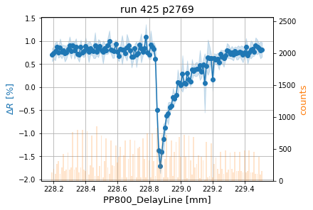
The output is an xarray.Dataset that contains the binned deltaR, its standard deviation and standard error, as well as the delay line position bins and the counts per bin.
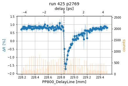
One can also convert the motor position axis in mm into temporal axis in ps. For this, the argument positionToDelay can be used, in combination with origin which gives the motor position for time zero and invert, which gives the sign of time axis relative to the motor axis. In this case, binWidth is the width in picosecond, and the output has a new coordinate delay_ps.
[2]:
refl = tb.reflectivity(ds, Iokey='FastADC5peaks', Irkey='FastADC3peaks',
                       delaykey='PP800_DelayLine',
                       positionToDelay=True, origin=228.845, invert=False,
                       binWidth=0.01, plot=True)
refl
[2]:
<xarray.Dataset>
Dimensions:                 (delay: 133)
Coordinates:
  * delay                   (delay) float64 228.2 228.2 228.2 ... 229.5 229.5
Data variables:
    FastADC5peaks           (delay) float64 2.009e+05 1.958e+05 ... 1.937e+05
    FastADC3peaks           (delay) float64 7.286e+04 6.932e+04 ... 7.36e+04
    FastADC5peaks_unpumped  (delay) float64 2.007e+05 1.955e+05 ... 1.935e+05
    FastADC3peaks_unpumped  (delay) float64 7.226e+04 6.872e+04 ... 7.293e+04
    PP800_DelayLine_binned  (delay) float64 228.2 228.2 228.2 ... 229.5 229.5
    deltaR                  (delay) float64 0.7039 0.7426 ... 0.8043 0.8176
    deltaR_std              (delay) float64 0.8555 0.9384 ... 0.9011 0.9902
    deltaR_stderr           (delay) float64 0.07418 0.06808 ... 0.09245 0.08032
    counts                  (delay) int64 133 190 114 266 304 ... 114 380 95 152
Attributes:
runFolder: /gpfs/exfel/exp/SCS/202201/p002769/raw/r0425- delay: 133
- delay(delay)float64228.2 228.2 228.2 ... 229.5 229.5
array([228.19, 228.2 , 228.21, 228.22, 228.23, 228.24, 228.25, 228.26, 228.27,
       228.28, 228.29, 228.3 , 228.31, 228.32, 228.33, 228.34, 228.35, 228.36,
       228.37, 228.38, 228.39, 228.4 , 228.41, 228.42, 228.43, 228.44, 228.45,
       228.46, 228.47, 228.48, 228.49, 228.5 , 228.51, 228.52, 228.53, 228.54,
       228.55, 228.56, 228.57, 228.58, 228.59, 228.6 , 228.61, 228.62, 228.63,
       228.64, 228.65, 228.66, 228.67, 228.68, 228.69, 228.7 , 228.71, 228.72,
       228.73, 228.74, 228.75, 228.76, 228.77, 228.78, 228.79, 228.8 , 228.81,
       228.82, 228.83, 228.84, 228.85, 228.86, 228.87, 228.88, 228.89, 228.9 ,
       228.91, 228.92, 228.93, 228.94, 228.95, 228.96, 228.97, 228.98, 228.99,
       229.  , 229.01, 229.02, 229.03, 229.04, 229.05, 229.06, 229.07, 229.08,
       229.09, 229.1 , 229.11, 229.12, 229.13, 229.14, 229.15, 229.16, 229.17,
       229.18, 229.19, 229.2 , 229.21, 229.22, 229.23, 229.24, 229.25, 229.26,
       229.27, 229.28, 229.29, 229.3 , 229.31, 229.32, 229.33, 229.34, 229.35,
       229.36, 229.37, 229.38, 229.39, 229.4 , 229.41, 229.42, 229.43, 229.44,
       229.45, 229.46, 229.47, 229.48, 229.49, 229.5 , 229.51])
- FastADC5peaks(delay)float642.009e+05 1.958e+05 ... 1.937e+05
array([200920.80827068, 195825.84736842, 189510.48684211, 188501.2406015 , 188378.09210526, 178347.77631579, 172510.37559809, 180592.78229665, 177619.125 , 188322.56725146, 188552.62128146, 182600.14327485, 179260.08133971, 173384.92105263, 181677.9122807 , 173940.15311005, 189150.84398496, 197525. , 192838.81578947, 192767.60588972, 200930.50292398, 192317.79605263, 189984.51476252, 187612.27368421, 187279.29554656, 182917.86984353, 188577.37559809, 183137.38815789, 187506.92748538, 187692.29605263, 197161.31359649, 186850.98079659, 191139.19298246, 183116.69736842, 185739.84586466, 181913.284689 , 190850.95614035, 189357.39314195, 180145.93117409, 187107.35087719, 182932.89927405, 178612.57894737, 197816.58421053, 181232.96710526, 186243.5877193 , 185072.10651629, 183689.51674641, 189223.09649123, 184499.76461988, 189261.23916409, 189302.44078947, 201999.93660287, 188284.12440191, 193327.71929825, 194833.64035088, 190444.93233083, 188375.27192982, 191503.24285714, 191733.3377193 , 193085.35964912, 188390.34210526, 200583.54489164, 191159.43859649, 191823.12753036, 188113.84375 , 192676.14473684, 196094.08133971, 194363.0430622 , 179547.44736842, 191910.14819945, 192854.11403509, 184552.23976608, 199775.16412742, 193359.28947368, 179800.69605263, 200066.39633174, 195319.82894737, 182674.09758772, 195655.54276316, 186347. , 188683.27339181, 194058.23421053, 193583.84210526, 196854.35387812, 201428.38815789, 194367.72368421, 194212.37055477, 206466.89164087, 202257.77894737, 191893.76973684, 192610.90191388, 183270.17293233, 195644.79949875, 192862.02631579, 188519.87763158, 191419.30959752, 192627.44736842, 186425.55509868, 182790.13157895, 190021.81578947, 193938.71052632, 197611.14035088, 185728.43421053, 203261.91689751, 198541.83947368, 206242.96929825, 184223.10087719, 186485.88947368, 196665.40789474, 191610.07578947, 186898.57142857, 190856.82748538, 190029.75858124, 193314.24736842, 205812.34210526, 196283.98574561, 204917.97368421, 204331.94736842, 184858.6622807 , 196732.83223684, 202482.06390977, 195409.64210526, 189902.76315789, 186521.84210526, 183957.52105263, 195779.66917293, 200891.96240602, 191778.62828947, 195179.25 , 195449.13596491, 184506.06052632, 190612.88421053, 193726.34210526]) - FastADC3peaks(delay)float647.286e+04 6.932e+04 ... 7.36e+04
array([72856.94736842, 69320.45789474, 65163.81578947, 65712.34962406, 65466.56578947, 59836.97368421, 56723.22488038, 60682.44617225, 63105.80592105, 68624.78947368, 65546.69908467, 62159.0877193 , 60646.50239234, 56972.43355263, 61569.13450292, 57006.35645933, 64891.44799499, 74590.20300752, 70388.3708134 , 69410.52506266, 74529.08479532, 69272.17434211, 67872.14762516, 67641.01578947, 65823.5951417 , 62037.55405405, 65903.47607656, 61076.13815789, 65717.6497076 , 64752.94736842, 70336.92982456, 64022.44736842, 65919.71929825, 62369.47532895, 63710.83383459, 61651.38755981, 65728.10526316, 65805.31259968, 59630.70242915, 65816.33991228, 63220.61433757, 59650.04035088, 75057.16710526, 62443.51785714, 65161.93859649, 64979.57769424, 63049.64114833, 67905.80701754, 63343.08625731, 67658.85758514, 66645.46710526, 75850.80502392, 65682.94417863, 70237.10526316, 70576.00584795, 68002.45394737, 65730.43859649, 68008.1593985 , 68256.3245614 , 69237.14035088, 66743.81983806, 74070.8250774 , 65874.04385965, 66345.39203779, 63851.84375 , 67526.69078947, 68314.92643541, 68100.3277512 , 57057.98684211, 64602.88642659, 66557.24561404, 62893.44005848, 72320.7098338 , 68318.89473684, 61111.61710526, 74585.01594896, 70878.75 , 63732.32017544, 70684.27549342, 66751.86842105, 68464.04605263, 70226.39078947, 69473.26315789, 73670.37811634, 74887.55526316, 75554.13157895, 71704.23897582, 76393.81733746, 72372.25789474, 67687.82090643, 68657.34210526, 63098.15037594, 72445.66165414, 71142.93421053, 67072.68157895, 69393.92260062, 66224.47368421, 64661.50575658, 59763.68421053, 66291.94078947, 69328.44482173, 74323.99122807, 66339.72180451, 75884.17313019, 75811.38684211, 80378. , 65301.96820175, 66485.62368421, 73480.75 , 69350.80526316, 68246.83458647, 69184.29239766, 70283.79405034, 71150.48421053, 79372.39473684, 70509.36184211, 80602.79934211, 78262.32894737, 63466.9627193 , 73199.79605263, 75885.94736842, 70899.70526316, 70328.36466165, 65183.76973684, 64047.02421053, 70102.63157895, 76442.21428571, 69687.48684211, 73643.92982456, 73165.25 , 66983.13289474, 70555.86315789, 73600.03289474]) - FastADC5peaks_unpumped(delay)float642.007e+05 1.955e+05 ... 1.935e+05
array([200694.83458647, 195514.69473684, 189227.92982456, 187790.19736842, 187953.26809211, 177604.73245614, 172034.61244019, 180130.63157895, 177259.54276316, 187929.04385965, 188007.41533181, 181952.4619883 , 178861.65550239, 172836.59473684, 181117.24853801, 173360.22488038, 188746.0858396 , 197224.45112782, 192317.35167464, 192330.67293233, 200344.16959064, 191837.80263158, 189574.24775353, 187415.01052632, 186859.79149798, 182356.79871977, 188098.89712919, 182419.07894737, 187010.6502924 , 186778.33552632, 196525.86842105, 186379.80369844, 190684.72807018, 182624.29111842, 185207.22857143, 181195.3062201 , 190059.79824561, 189051.35326954, 179828.0465587 , 186593.45175439, 182213.34482759, 178333.35438596, 197498.12368421, 180725.71616541, 185644.26315789, 184536.4235589 , 183362.29585327, 188552.94736842, 183860.20467836, 188857.51083591, 189332.57236842, 201740.62200957, 187716.30143541, 193076.52631579, 194376.00584795, 189818.75469925, 187266.53508772, 191055.23383459, 190971.43859649, 192383.68421053, 188091.2145749 , 200226.3993808 , 190363.00877193, 191284.71592443, 187636.53782895, 192679.59210526, 195681.7888756 , 194135.10047847, 179222.42434211, 191471.56648199, 191703.79824561, 183994.07017544, 199336.78878116, 192943.54385965, 179239.58552632, 199585.28628389, 194555.97368421, 182331.26425439, 195267.46052632, 185590.5877193 , 188152.98538012, 193465.84736842, 192769.02631579, 196444.60872576, 201143.46973684, 193225.85526316, 193947.40327169, 206039.19504644, 201794.16315789, 191361.20102339, 192294.14354067, 182721.53947368, 195173.45864662, 192232.57894737, 188264.06710526, 190931.79411765, 192739. , 186124.78865132, 182381.03508772, 189245.05263158, 193306.60950764, 197997.85964912, 185259.27255639, 202629.70498615, 197956.64473684, 205554.84210526, 183575.36513158, 185874.69736842, 196401.53947368, 191149.12842105, 185993.93609023, 190067.2748538 , 189583.86498856, 192791.53421053, 205283.07142857, 195779.65679825, 204519.40460526, 203922.07565789, 184360.11951754, 196346.75657895, 202086. , 194966.75368421, 189266.0075188 , 186279.40789474, 183627.37473684, 195389.94736842, 200592.60526316, 191638.30372807, 194755.84210526, 194759.74122807, 184065.14605263, 190230.07894737, 193532.18421053]) - FastADC3peaks_unpumped(delay)float647.226e+04 6.872e+04 ... 7.293e+04
array([72262.08646617, 68715.23947368, 64584.20175439, 64910.38157895, 64833.49342105, 59106.03947368, 56142.70574163, 60049.11363636, 62547.86513158, 67968.01461988, 64835.23340961, 61410.92397661, 60035.79425837, 56307.29210526, 60912.39181287, 56334.40669856, 64290.58145363, 73954.81954887, 69602.3062201 , 68747.07330827, 73756.76315789, 68501.36513158, 67171.10590501, 67085.43684211, 65139.84412955, 61356.56899004, 65240.95454545, 60270.40789474, 65060.14795322, 63931.81578947, 69509.25438596, 63370.50924609, 65276.53508772, 61682.54111842, 63032.59398496, 60885.36602871, 64811.21052632, 65174.12200957, 59047.29959514, 65140.74122807, 62407.18602541, 59100.0877193 , 74451.58157895, 61769.08082707, 64408.19298246, 64258.52005013, 62484.62679426, 67085.78947368, 62560.12573099, 66987.68343653, 66205.17763158, 75253.58732057, 64950.70414673, 69664.80701754, 69905.63840156, 67168.31109023, 64805.73684211, 67350.6481203 , 67421.03654971, 68223.87719298, 66152.13495277, 73418.97213622, 65013.28070175, 65595.4925776 , 63168.81085526, 67104.56578947, 68583.23624402, 68974.40909091, 57950.04605263, 65383.96952909, 66946.88596491, 63264.74561404, 72609.42243767, 68591.45614035, 61185.63552632, 74705.59888357, 70767.28947368, 63788.25328947, 70662.82401316, 66433.33333333, 68244.16008772, 69994.31710526, 69007.31578947, 73454.33448753, 74729.07894737, 74920.73684211, 71491.28307255, 76140.02167183, 71930.71578947, 67287.52997076, 68302.85167464, 62664.63909774, 72003.86716792, 70552.96052632, 66759.21842105, 68895.63931889, 66216.18421053, 64270.41036184, 59248.26315789, 65624.38815789, 68693.34974533, 74345.26315789, 65766.31390977, 75203.19806094, 75142.10789474, 79718.27631579, 64620.84758772, 65860.70789474, 72925.60087719, 68719.71052632, 67388.46992481, 68395.48538012, 69628.96453089, 70454.28947368, 78628.03007519, 69799.50109649, 79918.22368421, 77523.79605263, 62848.68969298, 72544.64802632, 75206.12030075, 70235.92421053, 69488.56390977, 64681.32236842, 63473.79578947, 69390.87218045, 75703.09398496, 69123.03508772, 72850.02631579, 72288.59649123, 66261.175 , 69864.12105263, 72929.83552632]) - PP800_DelayLine_binned(delay)float64228.2 228.2 228.2 ... 229.5 229.5
array([228.19, 228.2 , 228.21, 228.22, 228.23, 228.24, 228.25, 228.26, 228.27, 228.28, 228.29, 228.3 , 228.31, 228.32, 228.33, 228.34, 228.35, 228.36, 228.37, 228.38, 228.39, 228.4 , 228.41, 228.42, 228.43, 228.44, 228.45, 228.46, 228.47, 228.48, 228.49, 228.5 , 228.51, 228.52, 228.53, 228.54, 228.55, 228.56, 228.57, 228.58, 228.59, 228.6 , 228.61, 228.62, 228.63, 228.64, 228.65, 228.66, 228.67, 228.68, 228.69, 228.7 , 228.71, 228.72, 228.73, 228.74, 228.75, 228.76, 228.77, 228.78, 228.79, 228.8 , 228.81, 228.82, 228.83, 228.84, 228.85, 228.86, 228.87, 228.88, 228.89, 228.9 , 228.91, 228.92, 228.93, 228.94, 228.95, 228.96, 228.97, 228.98, 228.99, 229. , 229.01, 229.02, 229.03, 229.04, 229.05, 229.06, 229.07, 229.08, 229.09, 229.1 , 229.11, 229.12, 229.13, 229.14, 229.15, 229.16, 229.17, 229.18, 229.19, 229.2 , 229.21, 229.22, 229.23, 229.24, 229.25, 229.26, 229.27, 229.28, 229.29, 229.3 , 229.31, 229.32, 229.33, 229.34, 229.35, 229.36, 229.37, 229.38, 229.39, 229.4 , 229.41, 229.42, 229.43, 229.44, 229.45, 229.46, 229.47, 229.48, 229.49, 229.5 , 229.51]) - deltaR(delay)float640.7039 0.7426 ... 0.8043 0.8176
array([ 0.70385124, 0.74255221, 0.77766998, 0.87017641, 0.74800608, 0.86592472, 0.77128721, 0.80402254, 0.72950695, 0.75897156, 0.83430226, 0.91101336, 0.78813673, 0.90790016, 0.79596252, 0.87665395, 0.71683061, 0.71309442, 0.87295462, 0.75857596, 0.77615089, 0.89693514, 0.83722401, 0.7661077 , 0.83756665, 0.80458832, 0.78111814, 0.90833003, 0.76409443, 0.84349968, 0.887969 , 0.79121062, 0.76239562, 0.83904305, 0.80538514, 0.89965652, 1.00601237, 0.81416877, 0.80146468, 0.78085243, 0.93731413, 0.76565696, 0.66771189, 0.82960754, 0.80956486, 0.81472271, 0.7364535 , 0.86384325, 0.9037318 , 0.79830365, 0.6533153 , 0.66037838, 0.84896043, 0.71070147, 0.73876342, 0.92704938, 0.84830079, 0.76066275, 0.84390484, 1.09900499, 0.75314225, 0.7053432 , 0.91964663, 0.88049906, 0.8337061 , 0.61332073, -0.4908297 , -1.38092418, -1.71694534, -1.41272649, -1.12163788, -0.88495334, -0.62656642, -0.57221739, -0.43261207, -0.4023655 , -0.21184841, -0.25310234, -0.17742998, 0.0979598 , 0.0878335 , 0.04662353, 0.29446724, 0.08987701, 0.06824385, 0.31115536, 0.17084691, 0.12668076, 0.38790246, 0.34540416, 0.38015566, 0.39309014, 0.39800717, 0.47889755, 0.32988133, 0.48823219, 0.08986072, 0.45616356, 0.64689386, 0.6260554 , 0.63195432, 0.16682678, 0.62454736, 0.60145391, 0.61497957, 0.52936518, 0.71623744, 0.65510835, 0.62349348, 0.68527502, 0.79377491, 0.77646893, 0.72685078, 0.75086669, 0.71044156, 0.78726658, 0.73096593, 0.75446749, 0.77079654, 0.75317538, 0.71045167, 0.75575987, 0.8700996 , 0.68470576, 0.74954458, 0.81708488, 0.82238396, 0.77003303, 0.90494369, 0.87380964, 0.84730445, 0.80425014, 0.81763735]) - deltaR_std(delay)float640.8555 0.9384 ... 0.9011 0.9902
array([0.85545177, 0.93841195, 1.06069793, 0.97009039, 1.00235237, 1.02465659, 1.08881174, 1.18354284, 1.10105758, 0.94419448, 1.10333812, 1.25044795, 1.24834482, 1.38789353, 1.20968082, 1.34141326, 1.32929632, 0.96091553, 1.13292954, 1.25282489, 0.84890623, 1.14230059, 1.22441956, 1.11944006, 1.14878082, 1.25239186, 1.10905762, 1.2463384 , 1.09378785, 0.86490763, 0.9842779 , 0.97680361, 0.95354097, 1.11267323, 1.15434373, 1.31644897, 1.22174905, 1.13620792, 1.34936305, 1.12999776, 1.1443804 , 1.22406337, 1.10262927, 1.15136924, 1.22047518, 1.04570819, 1.03606003, 1.11332781, 1.25878664, 1.06410925, 1.01493852, 0.90763132, 1.18090303, 1.06900719, 1.08604532, 1.05785876, 1.21670241, 1.11325976, 0.92150781, 1.02190008, 1.17968835, 0.90456589, 1.19403934, 1.1603307 , 1.23112739, 1.16134584, 1.70470913, 1.56421405, 1.38444676, 1.28389825, 1.22478851, 1.2201193 , 0.99338145, 0.93029468, 1.12040987, 0.92498353, 0.85140904, 1.10356919, 0.91579844, 1.09458168, 1.02056374, 0.96768949, 0.88250351, 1.01015428, 0.95041354, 0.83544882, 1.11615574, 1.03195493, 1.09973941, 1.03368069, 1.06273812, 1.28234581, 0.96711403, 1.02144782, 1.17379835, 1.06847914, 1.42512259, 1.29904952, 1.47429674, 1.18975112, 1.18065232, 0.95923865, 0.94490389, 1.0050778 , 0.91978474, 0.82042184, 1.0577044 , 1.03664646, 0.9958693 , 1.01540754, 0.95103977, 0.97075627, 1.11194096, 0.99553242, 0.7820403 , 1.01667655, 0.84189865, 0.94093226, 1.12411352, 0.95974614, 1.02574266, 1.06979631, 1.15320017, 1.10202532, 1.14919617, 1.14551393, 0.91429609, 0.97152907, 0.93846568, 0.88445555, 1.02541101, 0.90108751, 0.99023653]) - deltaR_stderr(delay)float640.07418 0.06808 ... 0.09245 0.08032
array([0.07417708, 0.06807956, 0.09934346, 0.05948006, 0.05748885, 0.09596788, 0.07531468, 0.05788897, 0.08930756, 0.07220436, 0.05277982, 0.09562414, 0.08634982, 0.05034419, 0.0925066 , 0.0927875 , 0.04705658, 0.08332194, 0.07836638, 0.04434952, 0.06491748, 0.09265281, 0.04386938, 0.11485213, 0.07309517, 0.04723485, 0.07671512, 0.14296482, 0.03740676, 0.09921171, 0.0651854 , 0.03684085, 0.12629959, 0.06381619, 0.04476353, 0.09106068, 0.11442728, 0.04537577, 0.08585792, 0.07483593, 0.04875224, 0.07250726, 0.05656369, 0.04991819, 0.16165589, 0.05235089, 0.04137625, 0.14746387, 0.06806739, 0.04186682, 0.11642143, 0.0443937 , 0.04716072, 0.14159346, 0.04795007, 0.04586399, 0.16115617, 0.04317036, 0.04982944, 0.13535397, 0.04333693, 0.05033139, 0.15815437, 0.04262581, 0.07061 , 0.1332155 , 0.0589586 , 0.10819895, 0.07940347, 0.04778175, 0.1622272 , 0.0659765 , 0.03696983, 0.12322054, 0.05747581, 0.03694028, 0.09766331, 0.05167936, 0.03714053, 0.14498089, 0.03902223, 0.04964142, 0.20246019, 0.03759405, 0.04875519, 0.13552769, 0.04209661, 0.05741951, 0.11283088, 0.03952377, 0.07351113, 0.07862567, 0.04841626, 0.16570072, 0.06021459, 0.05945177, 0.32694554, 0.05268341, 0.19527537, 0.13647381, 0.04864793, 0.12705426, 0.05793577, 0.05289883, 0.0667282 , 0.07683955, 0.04953155, 0.07520624, 0.09327171, 0.04659009, 0.08246561, 0.07423559, 0.05319135, 0.07222351, 0.06781149, 0.04761024, 0.068287 , 0.07631968, 0.05264144, 0.07784569, 0.08894317, 0.04908562, 0.09999514, 0.08938606, 0.05272874, 0.09932866, 0.07927953, 0.04549602, 0.08789536, 0.08283685, 0.05260248, 0.09244963, 0.08031879]) - counts(delay)int64133 190 114 266 ... 114 380 95 152
array([133, 190, 114, 266, 304, 114, 209, 418, 152, 171, 437, 171, 209,
       760, 171, 209, 798, 133, 209, 798, 171, 152, 779,  95, 247, 703,
       209,  76, 855,  76, 228, 703,  57, 304, 665, 209, 114, 627, 247,
       228, 551, 285, 380, 532,  57, 399, 627,  57, 342, 646,  76, 418,
       627,  57, 513, 532,  57, 665, 342,  57, 741, 323,  57, 741, 304,
        76, 836, 209, 304, 722,  57, 342, 722,  57, 380, 627,  76, 456,
       608,  57, 684, 380,  19, 722, 380,  38, 703, 323,  95, 684, 209,
       266, 399,  38, 380, 323,  19, 608,  57,  76, 589,  57, 266, 361,
       190, 114, 456, 190, 114, 475, 133, 171, 437, 190, 133, 456, 152,
       152, 456, 152, 133, 475, 133, 152, 475, 133, 133, 456, 114, 114,
       380,  95, 152])
- runFolder :
- /gpfs/exfel/exp/SCS/202201/p002769/raw/r0425
Correction by the BAM
The BAM data can be taken into account by calculating the delay from the motor position and adding the BAM values to it:
[3]:
ds['delay'] = ds['BAM1932S'] + tb.positionToDelay(ds['PP800_DelayLine'], origin=228.845, invert=False)
Once this is done, the new delay variable has two dimensions trainId and sa3_pId, while the OL photodiodes (FastADC3peaks and FastADC5peaks) have dimensions trainId and ol_pId. The aligment of the OL pulses to the FEL pulses can be done by shifting the ol_pId coordinates:
[4]:
newds = tb.align_ol_to_fel_pId(ds)
newds
[4]:
<xarray.Dataset>
Dimensions:            (pulse_slot: 2700, sa3_pId: 38, trainId: 2222)
Coordinates:
  * sa3_pId            (sa3_pId) int64 542 582 622 662 ... 1902 1942 1982 2022
  * trainId            (trainId) uint64 1298104001 1298104002 ... 1298106265
Dimensions without coordinates: pulse_slot
Data variables:
    bunchPatternTable  (trainId, pulse_slot) uint32 2178857 0 2097193 ... 0 0 0
    PP800_DelayLine    (trainId) float64 229.1 229.1 229.1 ... 228.3 228.3 228.3
    BAM1932S           (trainId, sa3_pId) float32 -0.1843975 nan ... nan
    delay              (trainId, sa3_pId) float64 1.444 nan 1.468 ... -3.665 nan
    FastADC3peaks      (trainId, sa3_pId) float64 8.711e+04 ... 5.205e+04
    FastADC5peaks      (trainId, sa3_pId) float64 2.083e+05 ... 1.712e+05
Attributes:
runFolder: /gpfs/exfel/exp/SCS/202201/p002769/raw/r0425- pulse_slot: 2700
- sa3_pId: 38
- trainId: 2222
- sa3_pId(sa3_pId)int64542 582 622 662 ... 1942 1982 2022
array([ 542, 582, 622, 662, 702, 742, 782, 822, 862, 902, 942, 982, 1022, 1062, 1102, 1142, 1182, 1222, 1262, 1302, 1342, 1382, 1422, 1462, 1502, 1542, 1582, 1622, 1662, 1702, 1742, 1782, 1822, 1862, 1902, 1942, 1982, 2022]) - trainId(trainId)uint641298104001 ... 1298106265
array([1298104001, 1298104002, 1298104003, ..., 1298106263, 1298106264,
       1298106265], dtype=uint64)
- bunchPatternTable(trainId, pulse_slot)uint322178857 0 2097193 0 ... 0 0 0 0
array([[2178857, 0, 2097193, ..., 0, 0, 0], [2113321, 0, 2097193, ..., 0, 0, 0], [2113321, 0, 2097193, ..., 0, 0, 0], ..., [2113321, 0, 2097193, ..., 0, 0, 0], [2113321, 0, 2097193, ..., 0, 0, 0], [2113321, 0, 2097193, ..., 0, 0, 0]], dtype=uint32) - PP800_DelayLine(trainId)float64229.1 229.1 229.1 ... 228.3 228.3
array([229.08908844, 229.08906555, 229.088974 , ..., 228.31462097, 228.31329346, 228.31098175]) - BAM1932S(trainId, sa3_pId)float32-0.1843975 nan ... -0.1027241 nan
array([[-0.1843975 , nan, -0.16020365, ..., nan, -0.11839612, nan], [-0.21036915, nan, -0.18972209, ..., nan, -0.12564458, nan], [-0.16471547, nan, -0.16057302, ..., nan, -0.12399466, nan], ..., [-0.14423086, nan, -0.12761527, ..., nan, -0.13162898, nan], [-0.15879111, nan, -0.157679 , ..., nan, -0.12788105, nan], [-0.11632565, nan, -0.13366464, ..., nan, -0.1027241 , nan]], dtype=float32) - delay(trainId, sa3_pId)float641.444 nan 1.468 ... nan -3.665 nan
array([[ 1.44398529, nan, 1.46817914, ..., nan, 1.50998667, nan], [ 1.41786094, nan, 1.43850801, ..., nan, 1.50258552, nan], [ 1.46290386, nan, 1.4670463 , ..., nan, 1.50362467, nan], ..., [-3.68253887, nan, -3.66592329, ..., nan, -3.66993699, nan], [-3.70595535, nan, -3.70484324, ..., nan, -3.67504529, nan], [-3.67891193, nan, -3.69625092, ..., nan, -3.66531038, nan]]) - FastADC3peaks(trainId, sa3_pId)float648.711e+04 8.624e+04 ... 5.205e+04
array([[87111.5, 86240. , 84647. , ..., 63387.5, 60995. , 61653. ], [84728. , 86681.5, 86086. , ..., 61118. , 60375. , 60461. ], [88389. , 86537.5, 82353. , ..., 57068.5, 59046.5, 58784. ], ..., [73646. , 75065.5, 73397.5, ..., 51347.5, 49307.5, 48422.5], [69838.5, 70282. , 71442.5, ..., 48335. , 46444. , 48895.5], [76128. , 75253. , 76561. , ..., 51300. , 50681.5, 52051. ]]) - FastADC5peaks(trainId, sa3_pId)float642.083e+05 2.065e+05 ... 1.712e+05
array([[208281.5, 206494.5, 204945. , ..., 195133. , 191177. , 193192. ],
       [203924. , 205979.5, 205714.5, ..., 191344. , 190208.5, 190552.5],
       [210528. , 208069. , 203214.5, ..., 185302. , 190319.5, 189757. ],
       ...,
       [179038.5, 181458. , 181309.5, ..., 168465. , 165446.5, 163352.5],
       [177458.5, 177457. , 180836. , ..., 164743.5, 161151.5, 167133.5],
       [185155. , 184248.5, 186669. , ..., 168975. , 168502.5, 171166. ]])
- runFolder :
- /gpfs/exfel/exp/SCS/202201/p002769/raw/r0425
When plotting the reflectivity, one can use units='ps' to specify the correct units of the bottom axis (by default units='mm').
[6]:
refl = tb.reflectivity(newds, delaykey='delay', units='ps')
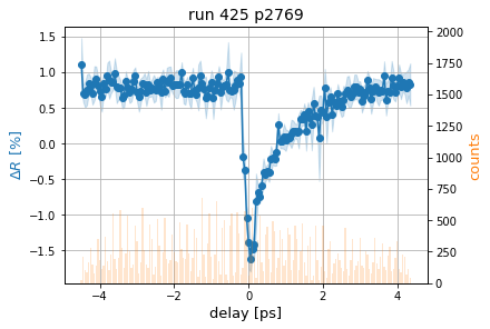
The shift in time corresponds to the BAM values, whose average in this run is newds['BAM1932S'].mean().values = -121.54 fs.