Data Correction
In this section, the procedure to update the offset calibration for the JUNGFRAU detector will be described, starting from the procedure to collect useful dark runs.
Dark runs acquisition
In order to fully characterize the offsets for the JUNGFRAU detector operating with dynamic gain switching, dark runs for all the three gain stages need to be acquired, in three separate runs, i.e. one run in Gain Mode: dynamic, one in forceswitchg1 and third in forceswitchg2. Each run must contain at least 500 trains of real data (i.e. non empty trains due to the DAQ running before the modules are sending out images). In order to maintain consistency with the constant map shape in the database, in the case of fixed gain operation three separate runs need to be acquired as well, i.e. in dynamic (as there is no fixg0 available), in fixg1 and fixg2. For the single cell operation these runs may be taken manually; however, since there is a JungfrauDarkChar middlelayer device deployed at each scientific instrument, the usage of this device is strongly encouraged, in order to minimize human error.
JungfrauDarkChar middlelayer
A middlelayer device with Class ID JungfrauDarkChar is deployed at each scientific instrument to automatize the dark run acquisition procedure for the JUNGFRAU detector. The currently deployed version works on a single detector, therefore a different instance is needed for each detector in operation, e.g. in the case of the scientific instrument FXE, there exist one instance for JF1M and a different instance for the JF500K. A version that can operate on more detectors simultaneously is currently under development.
Here a list of its relevant properties:
- Control device ids: list of the CONTROL devices it controls (typically one per instance);
- Receiver device ids: list of the RECEIVER devices it controls: these should be all the RECEIVERs referring to the one CONTROL in the previous property;
- DAQ controller id: self explanatory;
- Run controller id: self explanatory;
- Number of trains: number of train for each step of the process; default is 500;
The Run button starts the procedure; the detector should not be sending data while starting this, and the DAQ should be in MONITORING. The Cancel button halts the procedure in case it is needed, but clean reset somehow does not work and device shutdown and reinstantiation is needed in case of not proper termination.
The device will automatically recognize the detector operation mode from the settings in the CONTROL device by reading the properties Gain Mode, Exposure Time, Additional Storage Cells and Storage Cell Start (i.e. whether in burst or single cell, dynamic gain switching or fixed gain) and take dark runs accordingly, i.e. only for the current operation mode. It is therefore the responsibility of the operator to correctly configure the detector.
For example: if the CONTROL device is configured with Gain Mode: fixg2 and Additional Storage Cells: 15, the middlelayer will take dark runs for ‘Burst Mode - Fixed Gain’ operation only.
While taking runs, the device will also attempt to set the proper Run Type; it is therefore important that all the device properties named Experiment <operation> - <Gain Mode> are configured with Run Type name effectively present in the current proposal, otherwise the middlelayer will fail (additional empty spaces are relevant, unfortunately).
NOTE: as dynamic gain switching operation in burst mode is not supported, it is important to make sure that the detector is configured in Gain Mode: fixg1 or fixg2 before using the middlelayer, when operating it with 16 memory
cells.
Below the procedure to manually acquire darks is described. As explained before, it is recommended to use it only if problems with the JungfrauDarkChar middlelayer appear.
Single cell operation
Select the desired integration time in seconds (e.g. insert 1e-5 for 10 \(\mu s\));
assuming that the module is running in external trigger mode, select the number of trains, e.g. by setting Number of Trains = 1000 and Number of frames = 1;
select the desired gain stage:
- for the G0 darks, use the Gain Mode: dynamic and Setting: gain0,
- for the HG0 darks use the Gain Mode: dynamic and Setting: highgain0;
- for the G1 or G2 darks use forceswitchg1 or forceswitchg2 gain modes, respectively, when operating the detector in dynamic gain switching;
- the Gain Mode: fixg1 or fixg2 should be used for G1 and G2 if the detector is being operated in fixed gain;
take the run normally;
repeat for all the gain stages.
Burst mode operation
The current procedure to acquire dark runs in burst mode with dynamic gain switching operation is convoluted and it is not easily performed manually, so it won’t be described here. Additionally, this operation mode is currently not supported, therefore darks in this configuration should not be taken.
As for burst mode, fixed gain operation:
Select the desired integration time in seconds (e.g. insert 1e-5 for 10 \(\mu s\));
assuming that the module is running in external trigger mode, select the number of trains, e.g. by setting Number of Trains = 1000 and Number of frames = 1;
select the desired gain stage:
- for the G0 darks, use the Gain Mode: dynamic and Setting: gain0,
- for the HG0 darks use the Gain Mode: dynamic and Setting: highgain0;
- for the G1 or G2 darks use fixg1 or fixg2 gain modes, respectively;
take the run normally;
repeat for all the gain stages.
Remarks
A few final comments:
- the offset value depends from the integration time: if this parameter has been changed, it is necessary to repeat the dark runs acquisition;
- dark runs should be obviously repeated if the performances of the module changes, e.g. due to radiation damage;
- the stability of the offset depends from the thermal stability of the module: it is therefore suggested to let the module run for 10 - 15 min after power up and wait that it has thermalized, before taking darks and/or data.
Offsets injection
Once the dark runs for all the three gain stages have been acquired, it is possible to calculate new offset constants and inject them into the database by using a Jupyter notebook developed by the CAL team. This notebook accepts both dark runs for single cell mode and for burst mode (all the three of them must have been acquired in the same operation mode, though), and the Maxwell jobs running it can be launched directly from the myMdC page of your proposal. The procedure can be summarized in the following steps:
- migrate the three runs (G0, G1 and G2) to the Maxwell cluster;
- go to the Calibration Constants tab in the myMdC page of your proposal;
- under Detector select the desired JUNGFRAU detector;
- Under Run Number(s) input the run numbers for G0, G1 and G2 (in this order);
- click the Request button.
The notebook will require a few minutes (around 5 min) to terminate (for single-cell: darks in burst may require longer). After that, the newly calculated offset are injected into the database. A report is issued after the jobs are completed, and it can be downloaded from the same page.
In order to update also the online corrected preview, click on ‘Load Most Recent Constants’ from the calng MANAGER device.
As an example, typical results are also displayed below: on the left, the offset map for each gain stage, for 10 \(\mu s\) integration time.
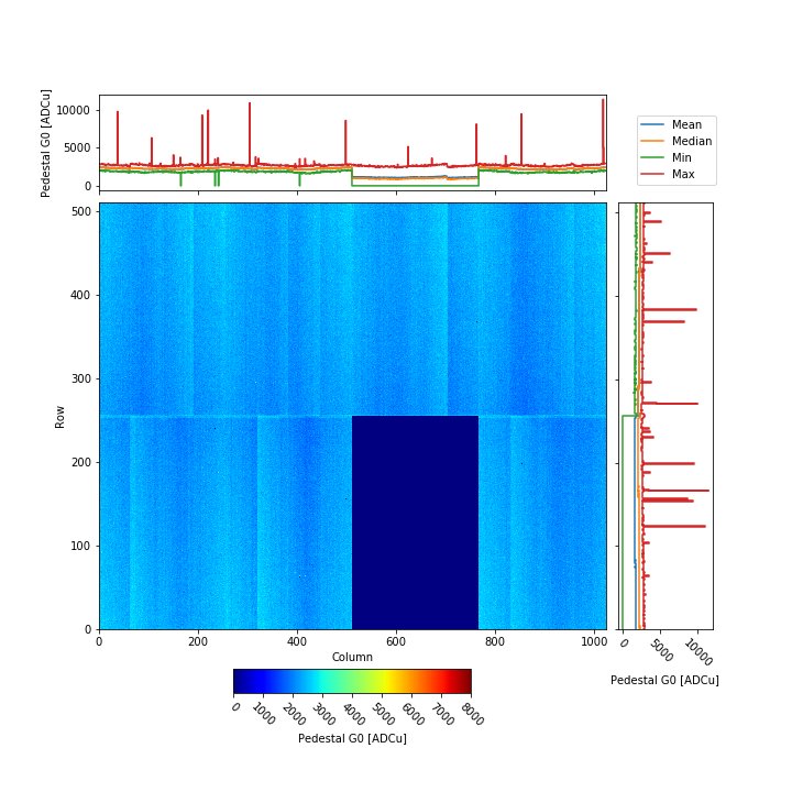
Fig. 13 Example of an offset map for G0; please note how the offset value lies around 2000 ADC units
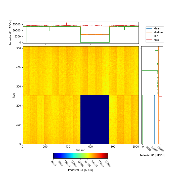
Fig. 14 Example of an offset map for G1; due to the signal inversion, the offset value is arounf 13000 ADC units
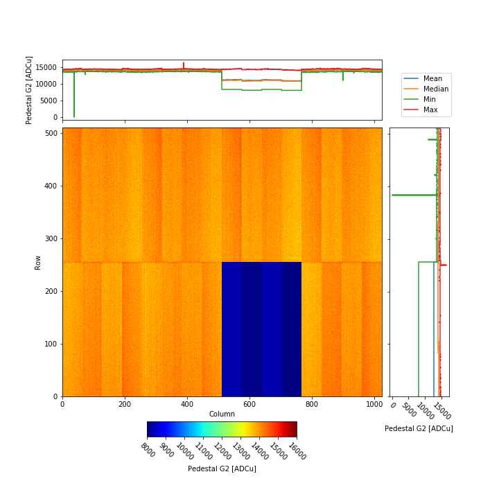
Fig. 15 Example of an offset map for G2; similar to the case of G1, due to signal inversion the offset value is again at the high end of the ADC range
Gain correction
There exist notebooks that use the offset and gain calibration constants present in the database, to convert the raw ADC output in physical units, how it has been outlined in subsection Raw data output. The recommended procedure is described in the section Calibration using the Metadata Catalogue Interface.
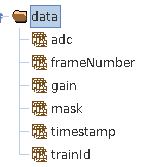
Fig. 16 The data structures that will be found in each hdf5 file, after calibration correction.
The notebook will create hdf5 files containing the corrected data using the currently available constants. In Fig. 16, the data structures that can be found in the hdf5 file containing the corrected data can be seen; they are similar to the data structures in the raw file, but with some differences:
- adc has the same shape of the data structure with the same name contained in the raw file (see Raw data output), but it now contains the corrected data, in keV units;
- mask is a new data structure and contains the map of the masked out pixels;
the remaining data structures are left unchanged.