There are plenty of resources in the litterature and on the web that introduce Gaussian optics and present the relevant quantities that need to be considered when dealing with such laser beams. Instead of making a redundant and incomplete presentation on Gaussian optics, this section shows important results from Gaussian optics applied to the practical cases of the laser beams encountered at SCS.

An introduction to Gaussian optics can be found on the Newport website

Another nice application note can be found on the Edmund Optics website.

Gaussian function

In Gaussian optics, it is convenient to define the Gaussian function as the following:

\[f(x) = I_0 \exp\left(-\frac{2(x-x_0)^2}{w_0^2}\right)\]

where \(w_0\) is the radius at \(1/e^2\), \(x_0\) is the center and \(I_0\) is the maximum amplitude. Note that \(w_0\) is equal to twice the standard deviation.

The full width at half-maximum (FWHM) is given by:

\[\frac{FWHM}{w_0} = \sqrt{2 \ln{2}} = 1.177\]

Or, alternatively:

\[\frac{w_0}{FWHM} = \frac{1}{\sqrt{2 \ln{2}}} = 0.849\]

The normalized intensity profile of a Gaussian beam is plotted below. The radii at several key percentages of intensity are indicated. For instance, in a pump-probe experiment, if we want to limit the variations of the pump beam intensity to 10%, the probe beam radius should be 23% that of the pump beam.

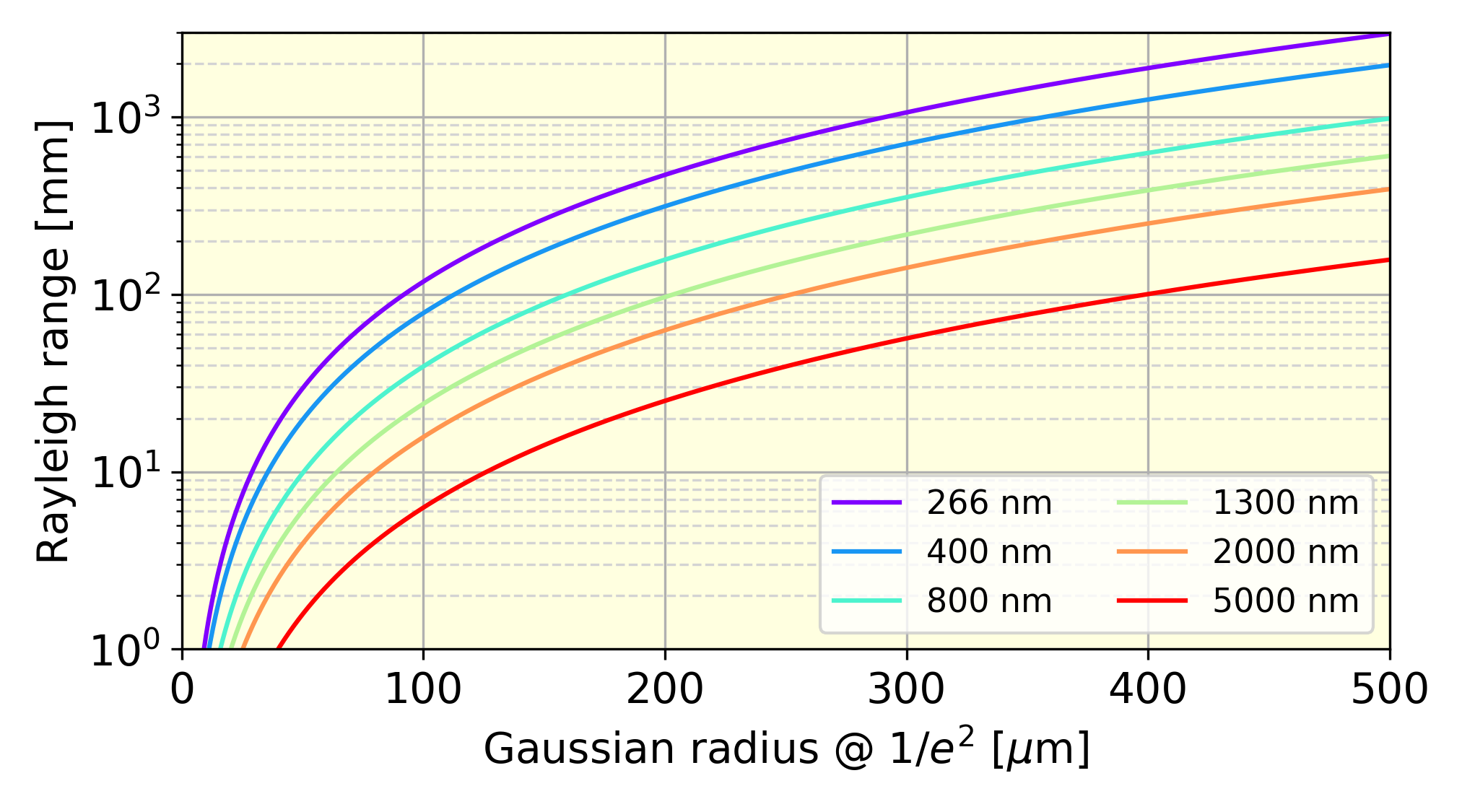
Rayleigh range

The Rayleigh range is the distance from the beam waist where the beam radius is increased by a factor \(\sqrt{2}\). For circular beams, this corresponds to an area increase by a factor 2. It is defined as:

\[z_R = \frac{\pi w_0^2}{\lambda}\]

with \(w_0\) the beam waist and \(\lambda\) the wavelength.

Typical Rayleigh ranges obtainable with the PP laser are plotted as a function of beam waist and wavelength below:

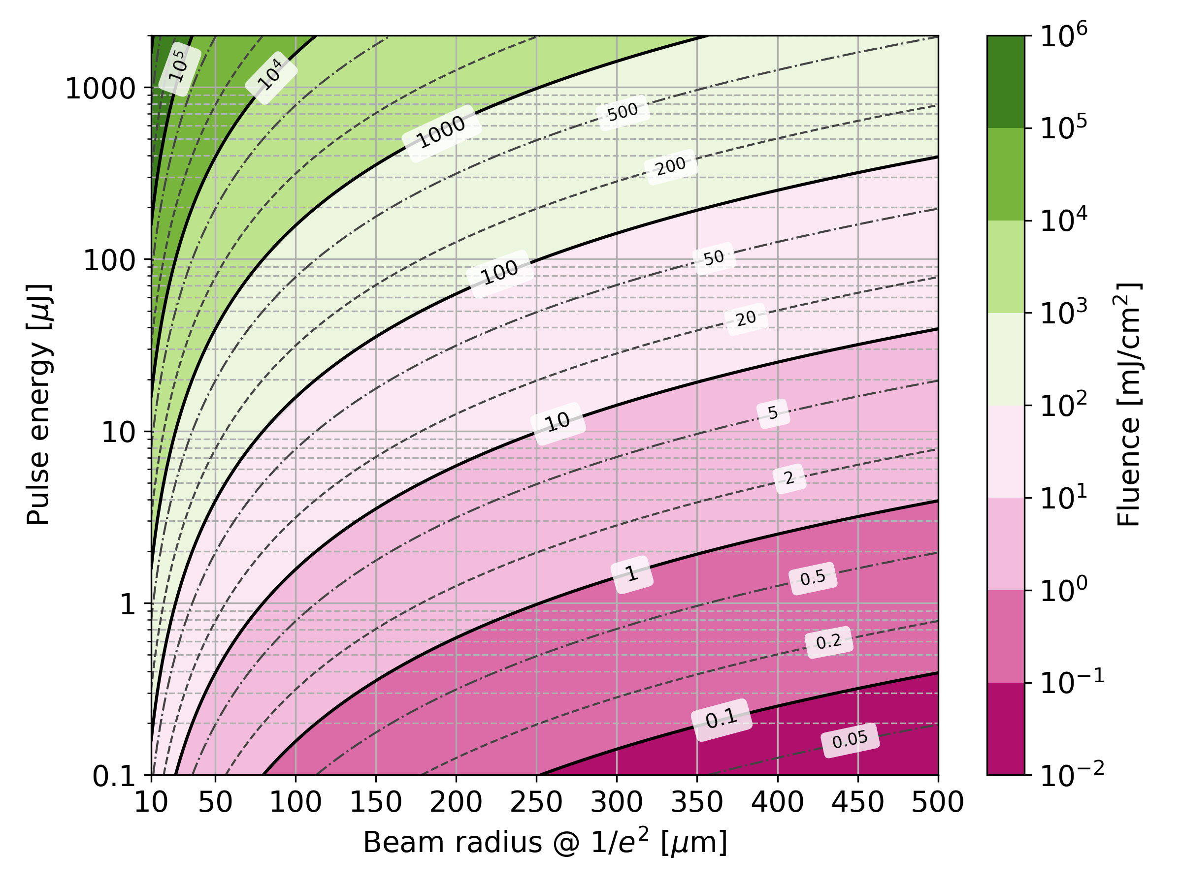
Peak fluence

The peak fluence of a pulsed Gaussian beam is defined as:

\[F_0 = \frac{2 E_P}{\pi w_{0,x} w_{0,y}}\]

with \(E_p\) the pulse energy, \(w_{0,x}\) and \(w_{0,y}\) the beam radii at \(1/e^2\) in x and y axes, respectively.

Using the full width at half maximum (\(D_x\) and \(D_y\)), the formula becomes:

\[F_0 = \frac{4 ln 2 E_P}{\pi D_x D_y}\]

Note

Sometimes, the fluence is calculated as \(E_P/(D_x D_y)\) where \(D\) is the FWHM. This definition is not the peak fluence of a Gaussian beam and is larger by a factor \(\pi/4\ln{2}=1.133\).

The following figure shows a map of fluence as a function of pulse energy and beam radius. The iso-curves for fluence at \(1\times10^n\), \(2\times10^n\) and \(5\times10^n\) mJ/cm² are shown in solid, dashed and dash-dotted lines, respectively.

The section below gives details of the derivation of the peak fluence.

For a Gaussian beam at the waist position, the intensity distribution is defined as:

\[I(x,y) = I_0 \exp{\left(-\frac{2x^2}{w_{0,x}^2} -\frac{2y^2}{w_{0,y}^2}\right)}\]

with \(I_0\) the peak intensity of the Gaussian beam, \(w_{0,x}\) and \(w_{0,y}\) the beam radii at \(1/e^2\) in x and y axes, respectively.

Let’s consider a knife-edge “corner” at position (x,y) that blocks the beam for \(x^\prime < x\) and \(y^\prime < y\). The detected power behind the knife-edge is given by:

\[P(x,y) = I_0 \int_{x}^\infty \int_{y}^\infty \exp{\left(-\frac{2x^{\prime 2}}{w_{0,x}^2} -\frac{2y^{\prime 2}}{w_{0,y}^2}\right)} dx^\prime dy^\prime\]

Now let’s consider a purely vertical knife-edge. The power in the y axis is integrated from \(-\infty\) to \(+\infty\), thus:

\[P(x) = I_0 \sqrt\frac{\pi}{2}w_{0,y}\int_x^\infty \exp{\left(-\frac{2x^{\prime 2}}{w_{0,x}^2}\right)}dx^\prime.\]

Similarly, for a purely horizontal knife-edge:

\[P(y) = I_0 \sqrt\frac{\pi}{2}w_{0,x}\int_y^\infty \exp{\left(-\frac{2y^{\prime 2}}{w_{0,y}^2}\right)}dy^\prime\]

By fitting the knife edge scans to these functions, we extract the waist in x and y axes.

The total power of one pulse is then:

\[P_{TOT} = \frac{I_0 \pi w_{0,x} w_{0,y}}{2}\]

Hence, the peak fluence, defined as \(F_0=I_0\tau\) with \(\tau\) the pulse duration of the laser, is given as:

\[F_0 = \frac{2 E_P}{\pi w_{0,x} w_{0,y}}\]

where \(E_P\) is the pulse energy.

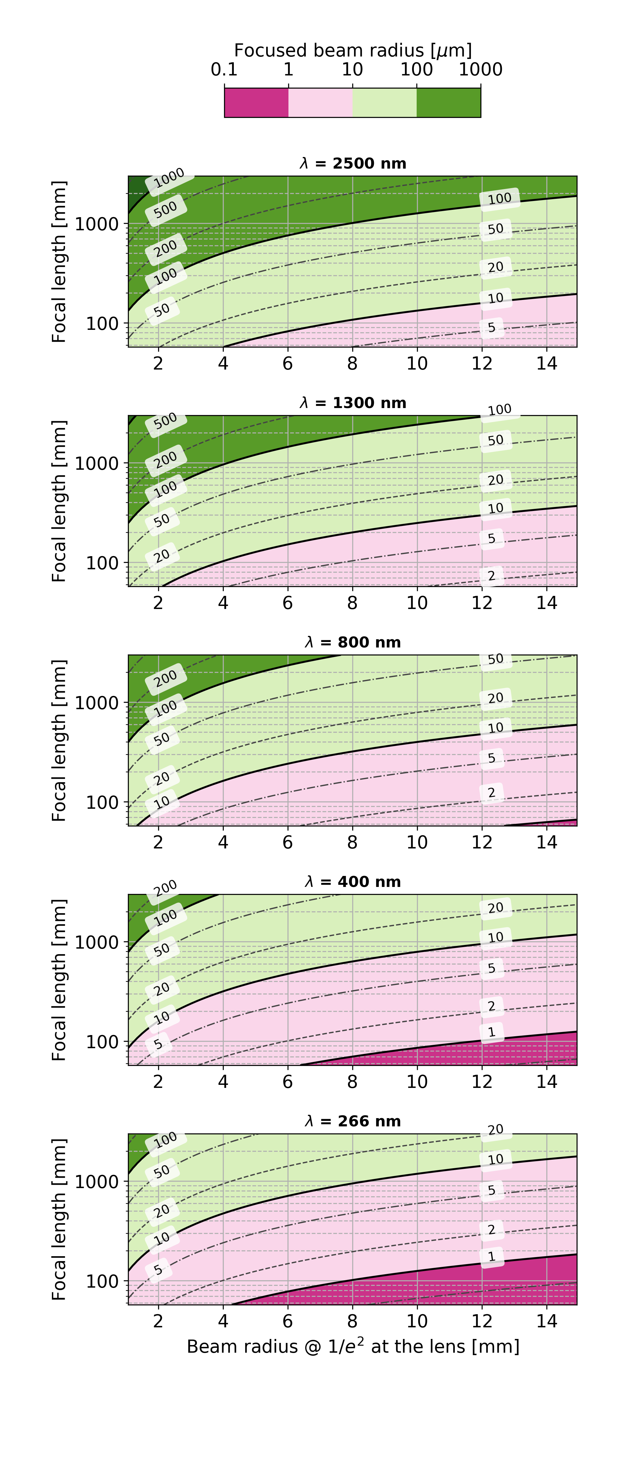
Focus by a thin lens

The equations that govern the waist position and size of a Gaussian beam focused by a thin lens can be simplified when the position of the lens is well within the Rayleigh range of the input beam. This approximation holds true for typical PP laser beam sizes, see Rayleigh range. The focus position is at the lens focal length and the size of the focused beam is given by the following formula:

\[w = \frac{\lambda f}{\pi w_0}\]

with \(w_0\) the radius of the input beam, \(\lambda\) the wavelength and \(f\) the focal length of the lens.

The following plots show maps of achievable focused beam radii for typical input beam radii and focal lengths, for the fundamental, second and third harmonic of the PP laser.